Grover’s Algorithm Step by Step: Quantum Search You Can Run on Real Hardware

What is Grover’s algorithm?

Grover’s algorithm is a quantum algorithm for searching an unstructured space of N possibilities. It finds a marked item in roughly √N steps, where a classical brute-force search needs about N checks on average.

That’s a quadratic speedup, not an exponential one and it isn’t a faster way to query a database. It’s a way to amplify the probability of a correct answer inside a quantum circuit, using an oracle you have to build yourself.

This article walks through how that amplification actually works, what breaks it if you run it too long, how to build it in Qiskit, and what happens the moment you move it off a simulator.

What problem does it actually solve? (And why “database search” is misleading)

Grover’s algorithm solves unstructured search: given a function that can check whether an item is the answer, find that item faster than checking every possibility one by one. It says nothing about how the item is stored.

Unstructured Search, Explained With a Real Example

Imagine a padlock with a 3-digit combination and a way to test any guess. With no other information, a classical approach checks combinations one at a time up to 1,000 tries in the worst case, 500 on average.

Grover’s algorithm reaches the correct combination in roughly √1000 ≈ 32 evaluations of the checking function, run as a quantum circuit instead of a loop. That’s the entire idea: fewer checks, not a smarter check.

Why It Isn’t a Database Search

A real database has indexes, sorted keys, and query planners , none of which Grover’s algorithm uses or needs. Calling it a “quantum database search” is where most explanations go wrong.

• A classical database with an index finds a record in roughly constant time, not N checks Grover’s speedup doesn’t apply there at all.
• Grover’s algorithm assumes the data isn’t indexed or sorted; it only assumes you can check a candidate.
• Getting classical data into a quantum state usable by Grover’s algorithm is itself a hard, often overlooked step , it isn’t free.

If you haven’t looked at how qubits and gates represent information yet, see [Internal link: Quantum Gates Explained] before this section the rest of this article assumes you know what a Hadamard gate and superposition are.

The Oracle Problem Nobody Mentions

Grover’s algorithm doesn’t work on raw data. It works on an oracle , a quantum circuit that recognizes the correct answer when it sees it.

Building that oracle is usually the hard part, and most introductions skip it entirely:

• The oracle has to be expressed as a reversible quantum circuit, not an ordinary function.
• For real problems (like inverting a cryptographic hash), the oracle itself can be enormous and deep.
• A slow, expensive oracle can erase the speedup Grover’s algorithm promises, since every iteration runs it at least twice.

Key takeaway: Grover’s algorithm is a multiplier on however good your oracle already is – it doesn’t replace the work of building one.

How does Grover’s algorithm work step by step?

Grover’s algorithm runs through five steps that repeat as a loop. Each one changes the quantum state in a specific, deliberate way, and the order matters.

1. Prepare the superposition
2. Mark the answer with the oracle
3. Amplify the marked state
4. Repeat
5. Measure

Step 1 : Put Every Possibility Into Superposition

What happens

The circuit starts with every qubit at 0, then a Hadamard gate is applied to each one. For n qubits, this creates an equal superposition across all 2ⁿ = N possible bitstrings.

Every candidate answer correct or not , now has exactly the same amplitude. Nothing has been “checked” yet; the circuit has just enumerated every possibility at once.

If Hadamard gates and superposition are new to you, [Internal link: Quantum Gates Explained] covers exactly what this gate does and why it produces an even mix rather than randomness.

Why it matters

This equal starting point is what makes the later steps meaningful. Amplification only works because every state begins on level footing.

Step 2 : The Oracle Marks the Answer

What happens

The oracle circuit runs once per iteration. It does not reveal the answer, print it, or collapse the state.

Instead, it flips the sign the phase of the amplitude belonging to the marked state. Every other amplitude stays untouched.

Nothing directly measurable has changed yet. If you measured right after this step, the odds of getting the marked state would be exactly what they were before: 1 in N.

Why it matters

A phase flip is invisible to a single measurement but very visible to the next step, the diffusion operator, which reacts to that sign difference. This is the same phase mechanic covered for single qubits in [Internal link: What Is the Bloch Sphere?] .Grover’s oracle is that idea applied across an entire register at once.

Before oracle	After oracle
All amplitudes positive, equal size	Marked amplitude flipped negative, same size
Measurement odds: 1/N for every outcome	Measurement odds: still 1/N for every outcome

Step 3 : The Diffusion Operator Amplifies It

What happens

The diffusion operator performs what’s usually described as “reflection about the average.” Picture every amplitude as a bar on a chart, and compute the average height of all the bars.

The marked bar is now negative (from Step 2), which pulls the average down slightly. Reflecting every bar about that average pushes the marked bar up further than any of the others move because it started on the opposite side of the average from everyone else.

Why it matters

This is the actual amplification. One pass doesn’t do much; it’s the repetition of oracle-then-diffusion that steadily grows the marked amplitude while shrinking the rest.

• Unmarked amplitudes: nudged slightly, staying close to their starting size
• Marked amplitude: grows noticeably larger with each pass
• Total probability across all states: still sums to 1 , amplification borrows from the crowd, it doesn’t create anything from nothing

For the mathematically curious

The diffusion operator is the transformation 2|s⟩⟨s| − I, where |s⟩ is the equal superposition state. Combined with the oracle’s phase flip, one oracle-plus-diffusion pass is a single Grover iteration, and each iteration rotates the state vector by a fixed angle θ = arcsin(1/√N) inside a two-dimensional subspace spanned by the marked and unmarked states.

Step 4 : Repeat About √N Times

What happens

Oracle, then diffusion, repeated. Each repetition rotates the state a little closer to the marked answer, following the same fixed angle from the box above.

The number of repetitions is not always exactly √N , the optimal count depends on N and is calculated per problem, not assumed.

Why it matters

Too few iterations and the marked state’s amplitude hasn’t grown enough. Too many, and as the next section covers in detail ,it starts shrinking again.

Step 5 : Measure

What happens

After the chosen number of iterations, every qubit is measured. This collapses the superposition into one classical bitstring, chosen according to each outcome’s probability.

If the iteration count was close to optimal, the marked answer is now by far the most likely single outcome but it’s still probabilistic, not guaranteed on any one run.

Why it matters

• Grover’s algorithm is normally run for many shots (repeated executions), not just once.
• The result is a distribution of outcomes, not a single guaranteed value.
• The marked bitstring should appear as the clear mode of that distribution when the circuit and iteration count are right.

Why do you have to stop Grover’s algorithm at the right number of iterations?

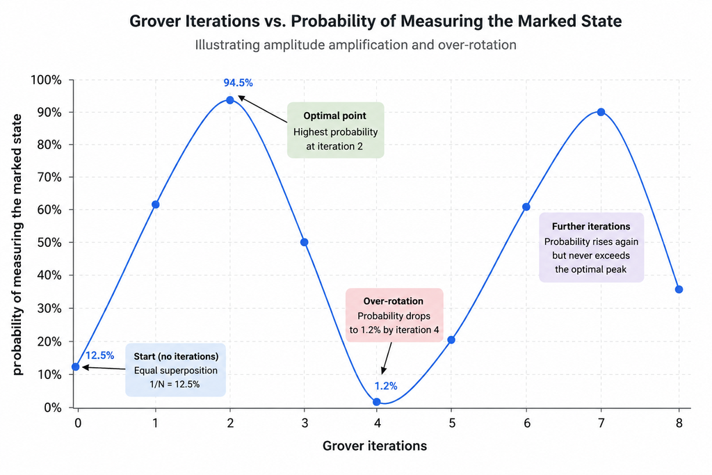
More iterations do not always mean a better result. Each Grover iteration rotates the state vector by a fixed angle toward the marked state and rotation doesn’t stop just because you’ve reached the best point.

Keep applying oracle-plus-diffusion past the optimal count, and the state rotates past the marked answer, sending the success probability back down. Run it long enough, and it swings low again before rising a second time.

This is often called over-rotation, and it’s the reason you can’t just “run Grover’s algorithm more” to be safer.

The chart below shows this for an 8-item search (3 qubits), using the exact probabilities produced by the simulation later in this article:

Iterations	Success probability
0	12.5%
1	78.1%
2 (optimal)	94.5%
3	33.0%
4	1.2%
5	54.8%

For the mathematically curious

The optimal iteration count is approximately ⌊(π/4)·√N⌋. For N = 8, that’s (π/4)·√8 ≈ 2.22, which rounds to 2 iterations matching the peak in the table above and confirmed by running the actual circuit later in this article. The exact success probability at k iterations is sin²((2k+1)θ), with θ = arcsin(1/√N).

How do you build Grover’s algorithm in Qiskit?

Qiskit version tested: 2.5.2, with qiskit-aer 0.17.2. Qiskit’s APIs change between major versions, so if you’re on an older install, some method names below may differ.

What You Need

• An IBM Quantum account (free tier is enough to try real hardware later)
• A browser-based notebook, or Python installed locally
• Basic Python, no GPU, and no physics background required
• pip install qiskit qiskit-aer

If you haven’t set up Qiskit before, [Internal link: Qiskit Tutorial] covers installation and your first circuit in more depth than repeated here.

The Oracle Circuit

The example below marks the bitstring 101 inside a 3-qubit search space (N = 8). The trick: temporarily flip the qubits that should read 0, so a single multi-controlled operation only fires on the target bitstring, then flip them back.

• X gates on any qubit that should be 0 in the target string, turning “match this pattern” into “match all-ones”
• A multi-controlled Z, built here from Hadamard-MCX-Hadamard, which flips the phase only when every qubit reads 1
• The same X gates again, undoing the temporary flip so the rest of the circuit is unaffected

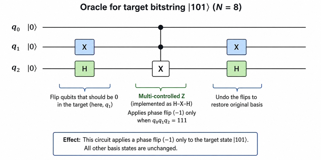
Oracle circuit marking the bitstring 101. Alt text: three-qubit quantum circuit with X gates, a controlled operation, and Hadamard gates forming a phase-flip oracle.

The diffusion operator follows the same H–X–controlled-Z–X–H pattern, but across every qubit, reflecting the whole state about its average:

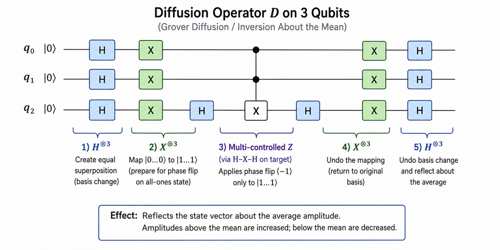
Diffusion operator on 3 qubits. Alt text: quantum circuit diagram showing the Grover diffusion operator built from Hadamard, X, and controlled-X gates.

The Full Program, End to End

This is the exact script used to generate every number in this article it was run, not written from memory.

# Grover’s algorithm on 3 qubits, marking the bitstring “101”

# Tested on Qiskit 2.5.2 + qiskit-aer 0.17.2

import math

from qiskit import QuantumCircuit, transpile

from qiskit_aer import AerSimulator

n = 3                 # number of qubits -> N = 2**n possibilities

marked = “101”       

# the answer Grover’s algorithm should find

def oracle(qc, marked_bitstring):

 # Flip qubits that should read 0, so the multi-controlled

 # operation below only triggers on the marked bitstring

    for i, bit in enumerate(reversed(marked_bitstring)):

        if bit == “0”:

            qc.x(i)

    qc.h(n – 1)

    qc.mcx(list(range(n – 1)), n – 1)   # multi-controlled X

    qc.h(n – 1)                 # H-MCX-H = multi-controlled Z

    for i, bit in enumerate(reversed(marked_bitstring)):

        if bit == “0”:

            qc.x(i)

def diffuser(qc, n):

    qc.h(range(n))

    qc.x(range(n))

    qc.h(n – 1)

    qc.mcx(list(range(n – 1)), n – 1)

    qc.h(n – 1)

    qc.x(range(n))

    qc.h(range(n))

# Calculate the optimal number of iterations for this N

N = 2 ** n

iterations = round((math.pi / 4) * math.sqrt(N))

print(“Optimal iterations:”, iterations)   # -> 2

# Build the circuit

qc = QuantumCircuit(n, n)

qc.h(range(n))                       # Step 1: superposition

for _ in range(iterations):

    oracle(qc, marked)               # Step 2: mark the answer

    diffuser(qc, n)                  # Step 3: amplify it

qc.measure(range(n), range(n))       # Step 5: measure

# Run on the simulator

sim = AerSimulator()

tqc = transpile(qc, sim)

result = sim.run(tqc, shots=2048).result()

counts = result.get_counts()

print(counts)

Running this script prints Optimal iterations: 2, matching the calculation in the previous section, and produces this measurement distribution over 2,048 shots:

{‘110’: 20, ‘111’: 20, ‘011’: 15, ‘100’: 12, ‘000’: 12, ‘010’: 18, ‘001’: 13, ‘101’: 1938}

The marked bitstring 101 was measured 1,938 out of 2,048 times about 94.6%, matching the 94.5% theoretical peak from the earlier table almost exactly.

Reading the Output

Qiskit returns counts, not a single answer , a histogram of how often each bitstring was measured across all shots.

• Shots: how many times the circuit was executed; more shots give a cleaner distribution but take longer
• Most frequent result: the bitstring with the highest count is your answer — 101 here, correctly
• The other bitstrings: small counts spread across wrong answers are expected, not a bug ,Grover’s algorithm makes the right answer likely, not certain on every run

What happens when Grover’s algorithm runs on real quantum hardware?

Everything above ran on a simulator, which behaves exactly like the maths predicts. Real hardware doesn’t.

Simulator vs Real QPU

	Simulator	Real QPU
Behavior	Ideal, matches the theoretical probabilities	Subject to gate errors, noise, and decoherence
Multi-controlled gates	Free, instant	Decomposed into many physical two-qubit gates, each with error
Repeatable	Identical distribution every run	Distribution shifts run to run and over time

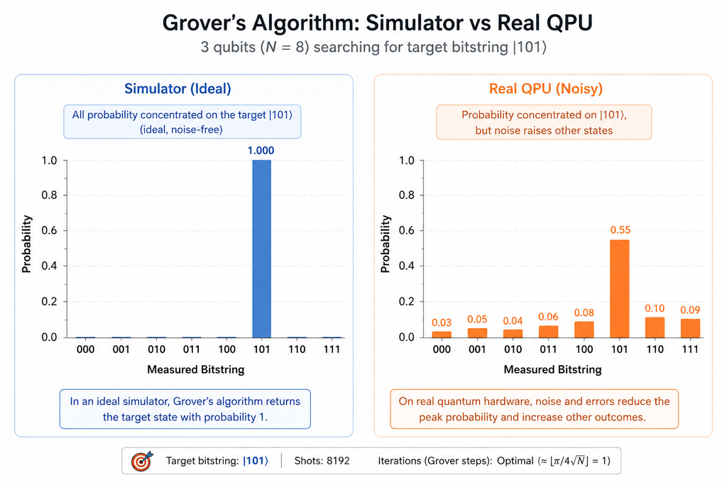
What the Results Look Like on a Real Machine

On current hardware, the oracle’s multi-controlled gates get compiled down into long chains of physical two-qubit gates and every one of those gates introduces a small chance of error.

• The marked bitstring’s probability shrinks compared to the clean simulator result.
• Incorrect bitstrings that should be near-zero start showing up with real, non-trivial counts.
• Deeper circuits (larger N, more iterations) accumulate more noise, compounding the problem.
• For a non-trivial example, more qubits than the toy case here – the correct answer may not come back as the single most frequent result.

Why It Doesn’t Scale Yet

The core issue is circuit depth. Grover’s algorithm needs the oracle and diffuser applied repeatedly, and every repetition adds more gates for noise to act on.

IBM’s own Qiskit and Quantum Learning documentation walks through exactly this trade-off between circuit depth and hardware error rates when running amplitude-amplification circuits worth reading directly rather than relying on secondhand summaries, since specific error-rate figures change as hardware improves.

What Does Fault Tolerant Mean and Why Is Grover’s Waiting for It?

Fault-tolerant quantum computing means a machine can detect and correct its own errors faster than they build up, using extra qubits dedicated to error correction rather than computation. Grover’s algorithm and most other quantum algorithms with real-world problem sizes needs that kind of reliability to run deep, wide circuits without the answer drowning in noise. For how that error correction actually works, see [Internal link: Quantum Error Correction Explained].

Where does Grover’s algorithm actually matter? Cryptography

Grover’s algorithm’s most concrete, well-established application isn’t search in the abstract , it’s brute-forcing symmetric encryption keys.

It Halves the Strength of Symmetric Encryption

Symmetric encryption (like AES) is typically attacked by brute-force key search trying keys until one works. That’s exactly the unstructured search problem Grover’s algorithm accelerates.

For a key of length k bits, a classical brute-force attack needs roughly 2^k attempts. Grover’s algorithm, run on a sufficiently large, fault-tolerant quantum computer, brings that down to roughly 2^(k/2).

This is usually summarized as: a 128-bit key has roughly 64 bits of effective security against an idealized large-scale quantum attack. That’s a simplified security-strength comparison, not a literal countdown to a specific date, no machine anywhere near this capability exists today.

Why AES-256 Is the Recommendation

Doubling the key length compensates for the quadratic speedup. AES-256 has roughly 128 bits of effective security against a Grover-style quantum attack the same margin AES-128 currently has against classical attackers.

This is why AES-256 (not AES-128) shows up repeatedly in post-quantum security recommendations, and it’s a software-level decision, not a hardware upgrade.

Grover’s algorithm affects symmetric cryptography; Shor’s algorithm is the quantum threat to RSA and ECC.These are frequently confused, and they are not the same problem, the same algorithm, or the same fix. For how the RSA/ECC side of this actually plays out and what organizations are doing about it today see [Internal link: Quantum Key Distribution].

What to learn before Grover’s algorithm makes sense

Grover’s algorithm assumes you’re already comfortable with a handful of prerequisites. If any of these feel shaky, it’s worth backfilling before circuit-level explanations click.

• Python : reading and writing basic scripts
• Basic probability : what a probability distribution and an expected value are
• Comfort with vectors : enough to picture amplitudes as arrows, not master linear algebra
• Qubits and superposition : see [Internal link: What Is Quantum Computing?]
• Quantum gates, especially Hadamard and multi-controlled gates : [Internal link: Quantum Gates Explained]
• Basic quantum circuit concepts : reading a circuit diagram left to right, qubits as wires

Ready to go beyond individual quantum algorithms?

Grover’s algorithm is one piece of a much larger quantum computing stack. If you want to move from understanding quantum concepts to building and executing quantum systems, the Certification in Applied Quantum Computing & AI by CEP, IIT Delhi takes you through quantum foundations, Qiskit, core algorithms, optimisation, quantum hardware, cybersecurity and Quantum-AI-with hands-on labs and progressively built capstones. 

FAQs