Quantum Interference Explained: The Hidden Engine Behind Quantum Speed-Ups

Quantum Interference Explained: The Hidden Engine Behind Quantum Speed-Ups

Quantum interference is what happens when the probability amplitudes of different quantum paths or possibilities combine.

When amplitudes line up, they reinforce each other in constructive interference. When they point in opposite directions, they cancel in destructive interference.

Quantum computers put this effect to work.

Superposition spreads a register across many states, and quantum gates adjust each state’s amplitude and phase so wrong answers cancel and useful ones stand out.

Algorithms such as Grover’s search and the Deutsch–Jozsa algorithm depend on this. Interference is a key ingredient in many quantum speed-ups, but it does not make every quantum computation faster.

How does Quantum Interference Work?

Quantum interference occurs when probability amplitudes linked to different alternatives combine into one amplitude for the same outcome. Each amplitude carries a magnitude and a phase.

The relative phase decides whether amplitudes reinforce or cancel.

The final probability comes from the combined amplitude, not from adding individual probabilities, which produces two patterns: constructive and destructive interference.

What are Probability Amplitudes in Quantum Computing?

Probability amplitudes are the numbers quantum mechanics uses to calculate the odds of each measurement outcome. They are complex numbers with a magnitude (size) and a phase (direction).

Unlike ordinary probabilities, amplitudes can be positive, negative or complex. One rule links an amplitude to its probability:

P(x) = |αₓ|²

Here, P(x) is the probability of outcome x, and αₓ is its amplitude. The bars mean “magnitude,” so amplitudes of +0.6 and −0.6 both give a probability of 0.36.

That is why phase matters. It stays hidden in a single amplitude, but when two amplitudes combine, their phases decide whether they reinforce or cancel.

What is Constructive Interference?

Constructive interference occurs when amplitudes with compatible phases combine into a larger amplitude. A larger combined amplitude means a higher probability for that outcome.

For example, two paths that each contribute an amplitude of 0.5 combine to 1.0, giving a probability of |1.0|² = 1.

Quantum algorithms use this to boost useful results. Reinforcement is always relative, though: it applies to particular outcomes under particular circuit operations.

What is Destructive Interference?

Destructive interference occurs when amplitudes with opposing phases, such as +0.5 and −0.5, reduce or cancel each other. A combined amplitude of zero means that outcome has zero probability.

Quantum circuits use carefully designed gates to suppress unwanted outcomes this way. Nothing is destroyed: the state evolves under quantum rules, and probability shifts to other outcomes.

Key point: Quantum interference changes the distribution of measurement outcomes by changing how probability amplitudes combine.

What is the Difference Between Quantum Interference and Classical Interference?

Classical waves and quantum systems both show constructive and destructive interference, and phase shapes the result in both. The difference is what combines.

Classical interference combines physical wave fields.

Quantum interference combines probability amplitudes that set measurement odds, and it appears even when each event is detected as a discrete click.

That does not make a particle a tiny classical wave. The table below compares the two across six features, from what combines to how each is used in computing.

Feature	Classical interference	Quantum interference
What combines	Physical wave fields or amplitudes	Quantum probability amplitudes
Role of phase	Changes the resulting wave	Changes the combined quantum amplitude
Observable result	Changes in wave intensity or field strength	Changes in measurement probabilities
Common example	Overlapping light or sound waves	Single-photon interference or quantum circuit outcomes
Measurement	Often measures a field or intensity	Produces outcomes with probabilities set by the quantum state
Role in computing	Used in optical and signal-processing systems	Used in quantum algorithms to shape outcome probabilities

How is Quantum Interference Different From Ordinary Probability?

In ordinary probability, if an event can happen in two mutually exclusive ways that nobody distinguishes, you add their probabilities.

Quantum mechanics changes that rule for coherent alternatives. You add the amplitudes first and square the total afterwards. Compare the two calculations:

P = |α₁ + α₂|² versus P₁ + P₂ = |α₁|² + |α₂|²

They differ by an interference term, 2|α₁||α₂|cos φ, where φ is the phase difference. It is positive near 0° (constructive) and negative near 180° (destructive).

The term survives only while the paths stay coherent. If any physical record reveals which path occurred, it vanishes and ordinary addition returns.

Key point: Quantum interference arises from combining amplitudes, not merely from adding probabilities.

How does Quantum Interference Relate to Superposition?

Superposition lets a quantum state hold several basis-state components, each with its own amplitude. Interference decides how those components combine when later gates act on them.

Superposition alone gives no advantage, because measurement returns one random outcome. Gates must change amplitudes and phases so the components interfere in favour of the desired result.

Can a Qubit Be in a Superposition Without Showing Interference?

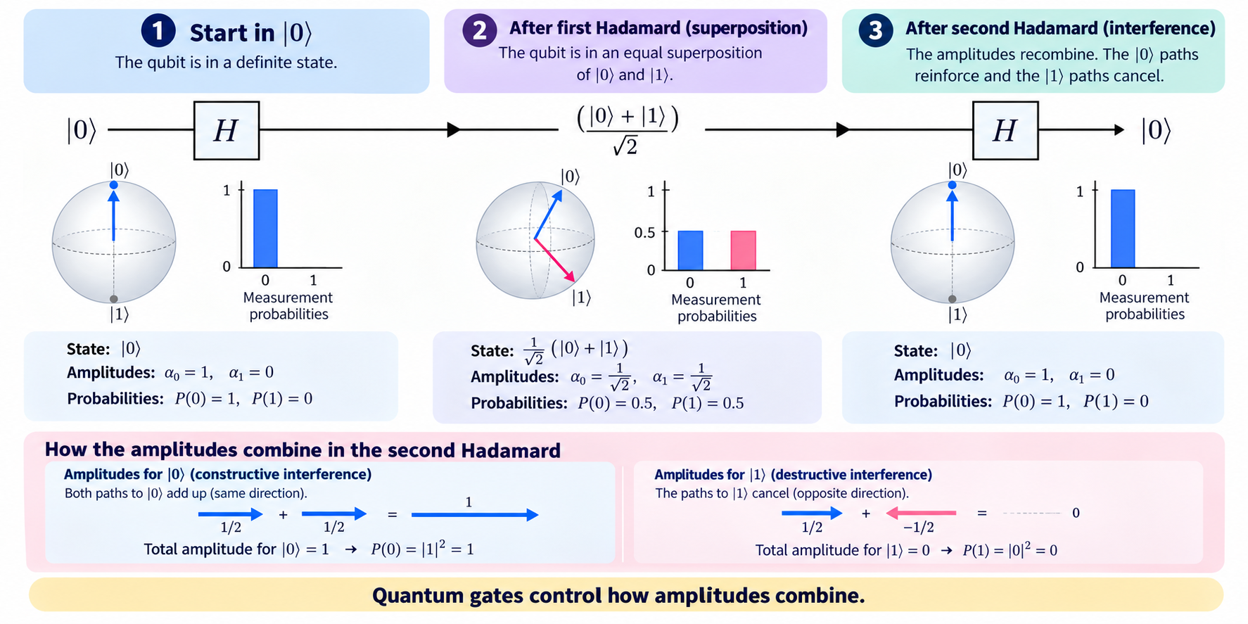
Yes. A qubit can sit in a superposition of |0⟩ and |1⟩ without showing interference, as long as nothing recombines its amplitudes.

The effect becomes visible only when a later gate brings the components back together. A Hadamard gate turns |0⟩ into the plus state:

|+⟩ = (|0⟩ + |1⟩) / √2

Measuring it in the computational basis gives 0 or 1 with probability 1/2 each, like a coin toss.

A second Hadamard gate recombines the amplitudes. Contributions to |0⟩ add (1/2 + 1/2 = 1) and contributions to |1⟩ cancel (1/2 − 1/2 = 0), so the qubit returns to |0⟩.

An equal classical mixture of 0 and 1 stays random after a Hadamard gate, because it has no fixed phase relationship to interfere.

Why do Quantum Gates Change Interference Patterns?

Quantum gates transform the amplitudes and phases of a state, so each gate reshapes the interference that later gates produce.

The Hadamard gate is the simplest example: it creates a superposition on one pass and recombines it on the next. Longer sequences can amplify some outcomes and suppress others.

Every gate must follow quantum mechanics’ rules. That means being reversible (unitary) and keeping total probability equal to 1.

How does Quantum Interference Enable Quantum Speed-Ups?

Quantum interference lets an algorithm raise the probability of useful outcomes and lower unhelpful ones.

Researchers Cleve, Ekert, Macchiavello and Mosca describe it as working “to enhance correct outcomes and suppress erroneous outcomes.” The speed-up comes from the whole algorithm, which shapes amplitudes over many steps around a problem’s structure.

The examples below are theoretical query-complexity advantages, counted in calls to a black-box function (an oracle). They are not guaranteed real-world runtime gains.

How does Quantum Interference Help Grover’s Search?

Grover’s algorithm searches an unstructured list of N items with about O(√N) oracle queries. Classical search needs O(N) queries in the worst case and about N/2 on average.

For one million items, that is roughly 785 Grover iterations versus about 500,000 classical lookups. The algorithm repeats a four-part interference cycle:

1. Superposition: Hadamard gates give every candidate the same amplitude.
2. Oracle: The target’s amplitude flips sign, a phase change that leaves its probability unchanged.
3. Diffusion: Every amplitude is reflected about the average, lifting the negative target amplitude well above the rest.
4. Repetition: About (π/4)√N iterations bring the target’s probability close to 1.

Too many iterations rotate probability away again. Grover’s query count is provably optimal for unstructured search, but it is not a general speed-up for searches with exploitable structure.

How does Interference Help the Deutsch–Jozsa Algorithm?

The Deutsch–Jozsa algorithm decides whether a promised Boolean function is constant (one output for all inputs) or balanced (0 for half the inputs, 1 for the rest).

A deterministic classical method may need 2ⁿ⁻¹ + 1 queries to be certain, or 513 for a 10-bit input. The quantum algorithm needs one, using three interference steps:

• Hadamard gates create an equal superposition of all 2ⁿ inputs.
• The oracle encodes each output as a phase, multiplying input x’s amplitude by (−1)^f(x).
• Final Hadamard gates recombine the amplitudes before measurement.

For a constant function, the amplitudes add and the all-zero string appears with certainty in the ideal algorithm.

For a balanced function, the all-zero amplitude cancels, so the result is a nonzero string.

This is a query-complexity result for a specific promise problem. Randomized classical methods can answer with high confidence in only a few queries.

Key point: Interference can create useful probability distributions, but the speed-up comes from how the algorithm exploits that behavior.

What is a Double-Slit Experiment, and How Does It Demonstrate Quantum Interference?

In the double-slit experiment, photons or electrons pass a barrier with two openings and strike a detection screen, even one at a time. Each lands as a single, localized dot.

Over many detections, bright and dark bands appear where amplitudes reinforced or cancelled. Reliable which-path information fades those bands.

The setup mirrors two computational paths recombining. It does not show particles computing every answer in parallel.

Why do Single Particles Produce an Interference Pattern?

Each particle has two coherent alternatives, the left and right slits, and both contribute amplitudes to every point on the screen.

Where those amplitudes arrive in phase, detection is likely. Where they arrive out of phase, it is unlikely.

In Akira Tonomura’s 1989 experiment, electrons sent one at a time gradually built clear fringes. The pattern is statistical, and it cannot come from particles colliding with each other.

What Happens When You Measure Which Path the Particle Takes?

Which-path information makes the alternatives distinguishable, so their amplitudes stop combining and the fringes fade.

Berthold-Georg Englert captured this trade-off in 1996 as D² + V² ≤ 1. D is path distinguishability and V is fringe visibility, so full path knowledge (D = 1) forces V = 0.

The effect depends on the physical interaction and measurement setup, not on a person looking. That is why quantum computers must preserve coherence.

What Limits Quantum Interference in Real Quantum Computers?

Quantum interference only works while a system keeps the coherence needed for amplitudes to combine as intended. Any disturbance to their phases changes the final probabilities.

In real hardware, noise and imperfect control blur the interference pattern and reduce algorithm accuracy. Three problems matter most:

• Decoherence: Environmental interactions scramble phase relationships.
• Gate errors: Slightly wrong rotations or phases make amplitudes recombine in the wrong proportions.
• Measurement errors: Readout sometimes reports the wrong result.

Error correction protects encoded information, while error mitigation uses repeated runs and post-processing to estimate and remove noise.

Better interference control is one part of building useful machines.

How does Decoherence Affect Quantum Interference?

Decoherence is the loss of coherent quantum relationships through interactions with the environment, such as heat, stray fields or vibration.

Once phase coherence leaks away, the interference an algorithm needs weakens or vanishes. Superconducting qubits are cooled near absolute zero and trapped ions are held in vacuum to limit this.

Deeper circuits take longer and accumulate more noise, which limits how accurate a computation can be.

Can Quantum Error Correction Preserve Interference?

Quantum error correction protects logical information by encoding it across many physical qubits. Peter Shor’s first scheme, in 1995, used nine physical qubits per logical qubit.

It measures only error syndromes, checks that reveal whether an error occurred, rather than the logical state. That keeps the phases interference depends on intact.

Longer computations also need fault-tolerant operations. The extra qubits and control mean error correction reduces errors without removing every practical challenge.

Key point: Quantum interference must be deliberately controlled and protected; it is not a guaranteed advantage simply because a system uses qubits.

What are the Common Misconceptions About Quantum Interference?

Simplified analogies help beginners picture quantum interference, but several leave the wrong impression. Most come from treating amplitudes like everyday waves or ordinary probabilities.

The table below pairs six common misconceptions with accurate explanations. It separates what interference does from what it does not imply.

Misconception	Accurate explanation
Quantum interference means a particle is literally a classical wave	Quantum states follow wave-like mathematics, but quantum objects are detected as discrete events and are not simply classical waves
Superposition means all answers can be read at once	Each measurement returns one outcome, so interference must concentrate probability on useful answers first
Interference always makes computation faster	It helps only when an algorithm arranges it around a problem’s structure
Destructive interference destroys information	It cancels amplitudes for particular outcomes within a reversible evolution; total probability is conserved
Quantum interference requires multiple particles	A single quantum system can interfere through its own coherent alternatives
Every quantum algorithm relies on the same interference pattern	Different algorithms use different operations, such as amplitude amplification in Grover’s search and phase encoding in Deutsch–Jozsa

Key point: Interference is a precise physical and mathematical phenomenon, not a general explanation for every claimed quantum advantage.

Key Takeaways: Quantum Interference Explained

Quantum interference is a precise mechanism, not a slogan for quantum power. It explains how algorithms shape outcomes and why noise limits them.

The points below condense how it works, how algorithms use it and what limits it in practice, as a quick reference:

• Quantum interference occurs when probability amplitudes combine.
• Constructive interference increases a combined amplitude; destructive interference reduces or cancels it.
• Quantum gates manipulate amplitudes and phases to shape measurement probabilities.
• Superposition creates combinations of states; interference determines how their amplitudes combine.
• Grover’s search and Deutsch–Jozsa use interference to support specific computational goals.
• Speed-ups depend on the problem, algorithm and hardware, not interference alone.
• Noise and decoherence weaken the coherence reliable interference needs.

Conclusion

Quantum interference remains one of the most important principles separating quantum computation from conventional approaches to information processing. Its long-term significance depends on whether researchers can translate precise control over quantum states into reliable computational advantages beyond carefully defined theoretical problems.

Progress in coherence preservation, error correction, and hardware design will be essential to making those advantages useful in practice. Understanding both the potential and the limitations of interference is therefore crucial to evaluating what quantum computers may realistically achieve.

Turn Your AI Knowledge into Practical Impact

Discover how AI can streamline workflows, strengthen data-driven decision-making, and improve operational efficiency with the Certificate Programme in AI-Powered Operations & Process Transformation by IIM Tiruchirappalli.

Explore the programme and learn how to apply AI to real-world operational challenges.

Frequently Asked Questions About Quantum Interference

How can quantum interference be demonstrated using a simple experiment?

A Mach–Zehnder interferometer is a simple demonstration. A beam splitter sends each photon along two paths, and mirrors recombine them at a second beam splitter.

Lengthening one path shifts the phase and moves detector counts from one exit to the other, even with single photons.

What is the role of phase in quantum interference?

Phase sets the relative direction of amplitudes, so it decides whether they add or cancel. Only relative phase matters; a global phase on the whole state changes nothing measurable.

Gates such as Z, S and T alter phase, which later gates convert into interference.

Why does quantum interference require coherence between quantum states?

Coherence means a state’s components keep a stable, well-defined phase relationship.

If phases drift randomly between runs, the interference term averages to zero. The state then behaves like a classical mixture, and outcome probabilities simply add, as they would for coin tosses.

How do quantum computers control probability amplitudes during a calculation?

They apply gate sequences, each delivered as a precisely timed pulse, such as microwaves for superconducting qubits or lasers for trapped ions.

Single-qubit rotations set amplitudes and phases. Two-qubit gates such as CNOT make one qubit’s amplitudes depend on another’s.

Can quantum interference be used to solve optimization problems?

In principle, yes. The Quantum Approximate Optimization Algorithm (QAOA) and Grover-based minimum finding use interference to bias results toward low-cost solutions.

Whether they beat the best classical optimizers on practical problems is still an open research question.

What is the relationship between quantum interference and quantum entanglement?

They are distinct but often work together. A single qubit can interfere with no entanglement, as the Hadamard example shows.

Entanglement makes amplitudes describe joint states of several qubits. Algorithms then make those joint amplitudes interfere, producing richer patterns.

How do researchers measure interference in a quantum circuit?

They run a circuit many times, each run called a shot, and compare outcome statistics with predictions.

A Ramsey-style sequence sweeps a phase between two Hadamard-like gates. The contrast of the resulting oscillation, its visibility, shows how much interference survived.

Why does observing a quantum system affect its interference behavior?

Observation means any physical interaction that records information, not a person looking.

The interaction entangles the system with a device or its environment, making the alternatives distinguishable. The interference term then vanishes, and probabilities revert to simple addition.

Can quantum interference occur in systems other than photons and electrons?

Yes. Neutrons, atoms and molecules interfere too. In 1999, Markus Arndt, Anton Zeilinger and colleagues observed interference of C60 molecules, made of 60 carbon atoms.

Their de Broglie wavelength of 2.5 picometres was roughly 400 times smaller than the molecule itself.

How is quantum interference used in quantum simulation?

Quantum simulation uses a controllable quantum system to model another, such as a molecule. Quantum phase estimation encodes a system’s energy as a phase.

Interference through the quantum Fourier transform then turns that phase into a readable binary number, revealing energy levels.

What is the difference between interference in quantum circuits and interference in quantum experiments?

The physics is identical; the setting differs. Experiments such as the double slit show interference across positions in space.

Quantum circuits create interference across bit strings in an abstract state space, using programmable gates in place of slits and mirrors.

How do scientists reduce noise to improve quantum interference in quantum processors?

Engineers combine better materials, shielding, cryogenic cooling and calibrated control pulses. Dynamical decoupling inserts pulse sequences that cancel slow phase drift.

Error mitigation corrects results statistically, and quantum error correction aims to remove errors faster than they accumulate.

Sources

Grover, L. K. (1996). A Fast Quantum Mechanical Algorithm for Database Search. Proceedings of the 28th Annual ACM Symposium on Theory of Computing, 212–219.

Boyer, M., Brassard, G., Høyer, P., & Tapp, A. (1996). Tight Bounds on Quantum Searching.

Bennett, C. H., Bernstein, E., Brassard, G., & Vazirani, U. (1997). Strengths and Weaknesses of Quantum Computing. SIAM Journal on Computing, 26(5), 1510–1523.

Deutsch, D., & Jozsa, R. (1992). Rapid Solution of Problems by Quantum Computation. Proceedings of the Royal Society of London A, 439, 553–558.

Then it will include the CTA of our program with its interlink.