Rod Cutting Problem

Problem Statement

Given a rod of length n  and array prices of length n denoting the cost of pieces of the rod of length 1 to n, find the maximum amount that can be made if the rod is cut up optimally.

Sample Test Cases

Input 1:

n = 8, prices[] = [1, 3, 4, 5, 7, 9, 10, 11]

Output 1:

12

Explanation 1:

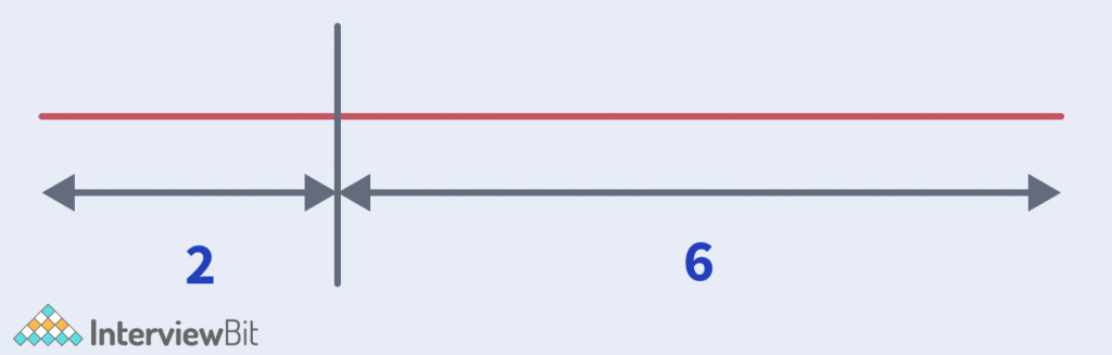
Cutting the rod into 2 rods of length 2 and 6 gives us a cost of 3 + 9  = 12, which is optimal.

Input 2:

n = 4, prices[] = [1, 1, 1, 6]

Output 2:

6

Explanation 2:

It can be seen that performing no cuts and taking the entire rod as a whole can lead to the optimal answer of 6.

Naive Approach

We can solve this problem naively with a recursive backtracking-based solution. By generating all possible configurations of different pieces and finding the maximum among them, we can get our optimal solution.

Code / Implementation:

C++ Code

int maximumProfit(vector < int > & prices, int n) {
  if (n == 0) {
    return 0;
  }
  int maxProfit = INT_MIN;
  for (int i = 1; i <= n; i++) {
    maxProfit = max(maxProfit, prices[i - 1] + maximumProfit(prices, n - i));
  }
  return maxProfit;
}

Java Code

 public static int maximumProfit(int[] prices, int n) {
   if (n == 0) {
     return 0;
   }
   int maxProfit = Integer.MIN_VALUE;
   for (int i = 1; i <= n; i++) {
     maxProfit = Math.max(maxProfit, prices[i - 1] + maximumProfit(prices, n - i));
   }
   return maxProfit;
 }

Python Code

def maximumProfit(prices, n):
    if n == 0:
        return n
    maxProfit = -999999
    for i in range(1, n + 1):
        maxProfit = max(maxProfit, prices[i - 1] + maximumProfit(prices, n - i))
    return maxProfit

Complexity Analysis:

• Time Complexity: Exponential
• Space Complexity: O(1) if recursion stack space is not considered

Memoization Based Approach

Considering the above recursion tree for n = 4, we can observe that there are multiple values, for which the function is being called again and again. Rather than using these redundant function calls, we can calculate the value of the function call once, and memoize it to use for future operations. Just by memoizing the results using an array or a hashmap, we can reduce the time complexity of the program from exponential to polynomial time complexity.

Now to memoize the function calls, into some relevant data structure, we need to find out our DP states. Here, we find from the above diagram that the overlapping subproblem depends only on the length of the current piece of the rod (n). So, our DP state will be the optimal cost which can be obtained if the length of the rod is n. This leads us to a 1D DP solution, which has,

• O(n) states
• O(n) time per transition  

Implementation:

C++ Code

int maximumProfit(vector < int > & prices, int n, vector < int > & dp) {
  if (n == 0) {
    return 0;
  }
  if (dp[n] != -1) {
    return dp[n];
  }
  int maxProfit = INT_MIN;
  for (int i = 1; i <= n; i++) {
    maxProfit = max(maxProfit, prices[i - 1] + maximumProfit(prices, n - i, dp));
  }
  return dp[n] = maxProfit;
}
int getMaxProfit(vector < int > & a, int n) {
  vector < int > dp(n + 1, -1);
  return maximumProfit(a, n, dp);
}

Java Code

public static int maximumProfit(int[] prices, int n, int[] dp) {
  if (n == 0) {
    return 0;
  }
  if (dp[n] != -1) {
    return dp[n];
  }
  int maxProfit = Integer.MIN_VALUE;
  for (int i = 1; i <= n; i++) {
    maxProfit = Math.max(maxProfit, prices[i - 1] + maximumProfit(prices, n - i, dp));
  }
  return dp[n] = maxProfit;
}
public static int getMaxProfit(int[] a, int n) {
  int[] dp = new int[n + 1];
  for (int i = 0; i <= n; i++) {
    dp[i] = -1;
  }
  return maximumProfit(a, n, dp);
}

Python Code

def maximumProfit(prices, n, dp):
    if n == 0:
        return n
    if dp[n] != -1:
        return dp[n]
    maxProfit = -999999
    for i in range(1, n + 1):
        maxProfit = max(maxProfit, prices[i - 1] + maximumProfit(prices, n - i, dp))
    dp[n] = maxProfit
    return dp[n]


def getMaxProfit(prices, n):
    dp = [-1] * (n + 1)
    return maximumProfit(prices, n, dp)

Complexity Analysis:

• Time Complexity: O(n²)
• Space Complexity: O(n)

Iterative Dynamic Programming Approach

Similar to the memoization approach, we can also solve this problem using tabulation-based Dynamic Programming. In any dynamic programming problem, there are 2 things that are to be considered,

• States: DP[i] = Best possible price for a rod of length i.
• Transitions: DP[i] = max(prices[j] + DP[i – j – 1]) overall values of j from [0, i – 1]

Using the above states and transitions, we can tabulate the optimal answer for all possible lengths of the rod, and finally, our required result will be stored in DP[n].

Implementation:

C++ Code

int maximumProfit(vector < int > & prices, int n) {
  vector < int > dp(n + 1, 0);
  if (n <= 0) {
    return 0;
  }
  int maxVal = INT_MIN;
  for (int i = 1; i <= n; i++) {
    for (int j = 0; j < i; j++) {
      maxVal = max(maxVal, prices[j] + dp[i - j - 1]);
    }
    dp[i] = maxVal;
  }
  return dp[n];
}

Java Code

public static int maximumProfit(int[] prices, int n) {
  int[] dp = new int[n + 1];
  if (n <= 0) {
    return 0;
  }
  int maxVal = Integer.MIN_VALUE;
  for (int i = 1; i <= n; i++) {
    for (int j = 0; j < i; j++) {
      maxVal = Math.max(maxVal, prices[j] + dp[i - j - 1]);
    }
    dp[i] = maxVal;
  }
  return dp[n];
}

Python Code

def maximumProfit(prices, n):
    dp = [0] * (n + 1)
    if n <= 0:
        return 0
    maxVal = -999999
    for i in range(1, n + 1):
        for j in range(i):
            maxVal = max(maxVal, prices[j] + dp[i - j - 1])
        dp[i] = maxVal
    return dp[n]

Complexity Analysis:

• Time Complexity: O(n²)
• Space Complexity: O(n)

Practice Problem:

• Rod Cutting

FAQs

Q.1: What is the time complexity per state transition of the Dynamic Programming approach?

Ans: The time complexity is O(n) per transition.

Q.2: How to identify that a problem can be solved by Dynamic Programming?

Ans: A problem can be solved using Dynamic Programming if it contains some Optimal Substructure and Overlapping Subproblems.