
Problem Statement
Travelling Salesman Problem (TSP)– Given a set of cities and the distance between every pair of cities as an adjacency matrix, the problem is to find the shortest possible route that visits every city exactly once and returns to the starting point. The ultimate goal is to minimize the total distance travelled, forming a closed tour or circuit.
The TSP is referred to as an NP-hard problem, meaning there is no known algorithm to solve it in polynomial time for large instances. As the number of cities increases, the number of potential solutions grows exponentially, making an exhaustive search unfeasible. This complexity is one of the reasons why the TSP remains a popular topic of research. Learn More.
Example 1: Travelling Salesman Problem
Input –
Confused about your next job?
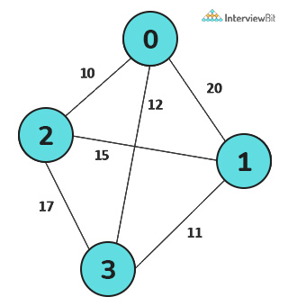
Output –
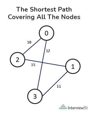
Here, the TSP Tour is 0-2-1-3-0 and the cost of the tour is 48.
Example 2: Travelling Salesman Problem
Input –
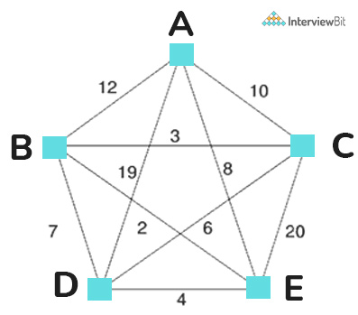
Output –
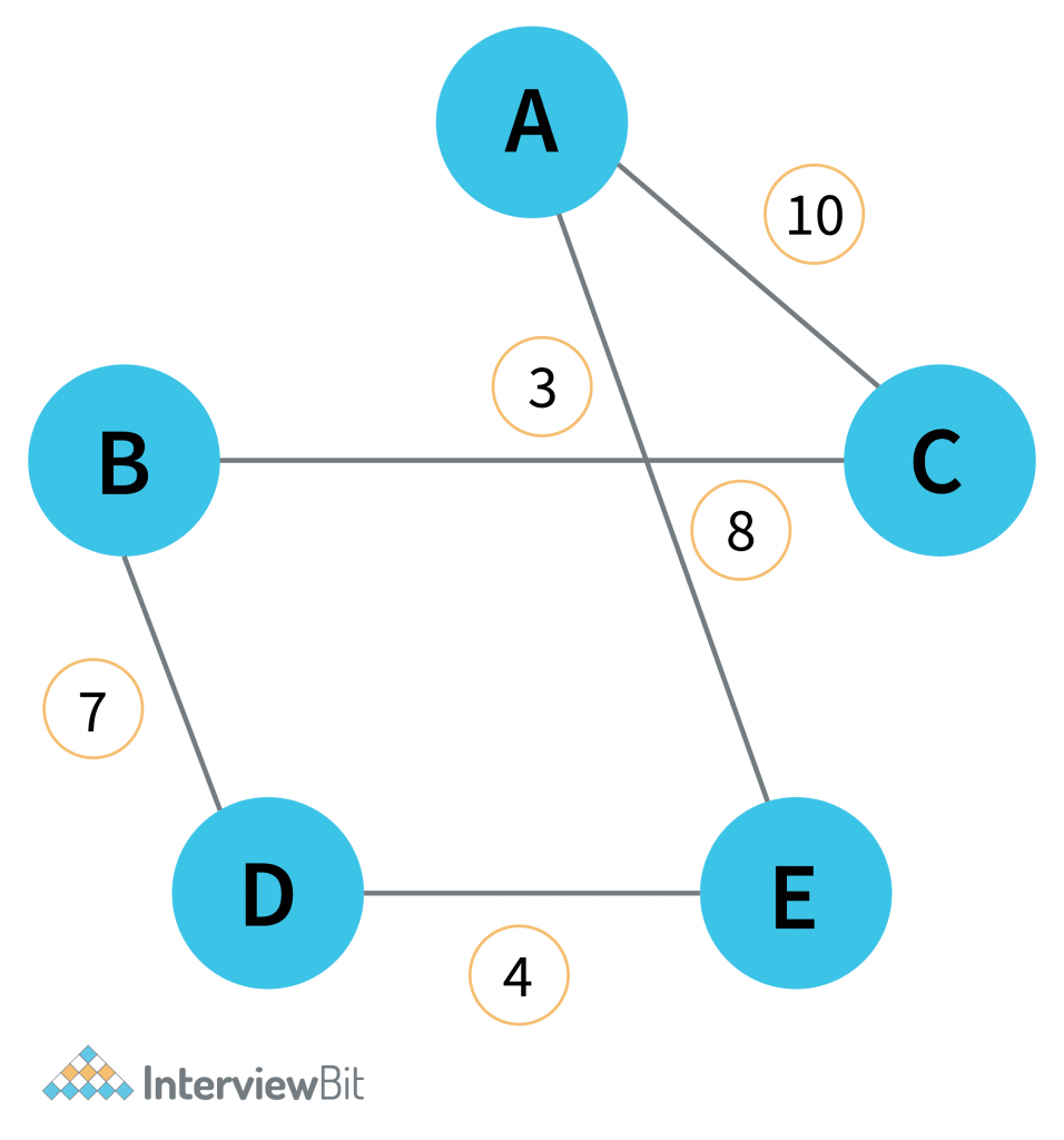
Minimum weight Hamiltonian Cycle: EACBDE= 32
Wondering how the Hamiltonian Cycle Problem and the Traveling Salesman Problem differ? The Hamiltonian Cycle problem is to find out if there exists a tour that visits each city exactly once. Here, we know that the Hamiltonian Tour exists (due to the graph being complete), and there are indeed many such tours. The problem is to find a minimum weight Hamiltonian Cycle.
There are various approaches to finding the solution to the travelling salesman problem- simple (naïve) approach, dynamic programming approach, and greedy approach. Let’s explore each approach in detail:
1. Simple Approach
- Consider city 1 as the starting and ending point. Since the route is cyclic, we can consider any point as a starting point.
- Now, we will generate all possible permutations of cities which are (n-1)!.
- Find the cost of each permutation and keep track of the minimum cost permutation.
- Return the permutation with minimum cost.
C++ Code Implementation
Java Code Implementation
Python Code Implementation
- Time complexity: O(N!), Where N is the number of cities.
- Space complexity: O(1).
2. Travelling Salesman Problem Using Dynamic Programming
In the travelling salesman problem algorithm, we take a subset N of the required cities that need to be visited, the distance among the cities dist, and starting cities s as inputs. Each city is identified by a unique city id which we say like 1,2,3,4,5………n
Here we use a dynamic approach to calculate the cost function Cost(). Using recursive calls, we calculate the cost function for each subset of the original problem.
To calculate the cost(i) using Dynamic Programming, we need to have some recursive relation in terms of sub-problems.
We start with all subsets of size 2 and calculate C(S, i) for all subsets where S is the subset, then we calculate C(S, i) for all subsets S of size 3 and so on.
There are at most O(n2^n) subproblems, and each one takes linear time to solve. The total running time is, therefore, O(n^22^n). The time complexity is much less than O(n!) but still exponential. The space required is also exponential.
C Code Implementation
C++ Code Implementation
Python Code Implementation
Java Code Implementation
- Time Complexity: O(N^2*2^N).
3. Greedy Approach
- First of all, we have to create two primary data holders.
- First of them is a list that can hold the indices of the cities in terms of the input matrix of distances between cities
- And the Second one is the array which is our result
- Perform traversal on the given adjacency matrix tsp[][] for all the cities and if the cost of reaching any city from the current city is less than the current cost update the cost.
- Generate the minimum path cycle using the above step and return their minimum cost.
C++ Code Implementation
Java Code Implementation
Python Code Implementation
- Time complexity: O(N^2*logN), Where N is the number of cities.
- Space complexity: O(N).
Practice Questions
Frequently Asked Questions
1. Which algorithm is used for the Travelling salesman problem?
Ans. Travelling Salesman Problem uses Dynamic programming with a masking algorithm.
2. What is the complexity of the Travelling salesman problem?
Ans.: The complexity of TSP using Greedy will be O(N^2LogN) and using DP will be O(N^22^N).
3. How is this problem modelled as a Graph problem?
Ans.: The TSP can be modelled as a graph problem by considering a complete graph G = (V, E). A tour is then a circuit in G that meets every node. In this context, tours are sometimes called Hamiltonian circuits.
4: What is the difficulty level of the Travelling salesman problem?
Ans.: It is an NP-hard problem.