Download PDF


Data structures are the building blocks of any computer program as they help in organizing and manipulating data in an efficient manner. Without data structures, the computer would be unable to understand how to follow a program's instructions properly. It also defines their relationship with one another.
Arrays, Linked Lists, Stacks, Queues, and others are examples of Data Structure. Data structures also provide clarity, organization and structure to the program's code while also helping the programmer ensure that each line of code performs its function correctly.

In this article, we've compiled the answers to the most frequently asked Data Structure Interview Questions so that you may better prepare for your job interview.
Basic Data Structure Interview Questions for Freshers
1. What are Data Structures?
A data structure is a mechanical or logical way that data is organized within a program. The organization of data is what determines how a program performs. There are many types of data structures, each with its own uses. When designing code, we need to pay particular attention to the way data is structured. If data isn't stored efficiently or correctly structured, then the overall performance of the code will be reduced.


 Real-Life Problems
 Prep for Target Roles
 Custom Plan Duration
2. Why Create Data Structures?
Data structures serve a number of important functions in a program. They ensure that each line of code performs its function correctly and efficiently, they help the programmer identify and fix problems with his/her code, and they help to create a clear and organized code base.
3. What are some applications of Data structures?
Following are some real-time applications of data structures:
- Decision Making
- Genetics
- Image Processing
- Blockchain
- Numerical and Statistical Analysis
- Compiler Design
- Database Design and many more
4. Explain the process behind storing a variable in memory.
- A variable is stored in memory based on the amount of memory that is needed. Following are the steps followed to store a variable:
- The required amount of memory is assigned first.
- Then, it is stored based on the data structure being used.
- Using concepts like dynamic allocation ensures high efficiency and that the storage units can be accessed based on requirements in real-time.
5. Can you explain the difference between file structure and storage structure?
- File Structure: Representation of data into secondary or auxiliary memory say any device such as a hard disk or pen drives that stores data which remains intact until manually deleted is known as a file structure representation.
- Storage Structure: In this type, data is stored in the main memory i.e RAM, and is deleted once the function that uses this data gets completely executed.
The difference is that the storage structure has data stored in the memory of the computer system, whereas the file structure has the data stored in the auxiliary memory.
 Learn via our Video Courses
6. Describe the types of Data Structures?
- Linear Data Structure: A data structure that includes data elements arranged sequentially or linearly, where each element is connected to its previous and next nearest elements, is referred to as a linear data structure. Arrays and linked lists are two examples of linear data structures.
- Non-Linear Data Structure: Non-linear data structures are data structures in which data elements are not arranged linearly or sequentially. We cannot walk through all elements in one pass in a non-linear data structure, as in a linear data structure. Trees and graphs are two examples of non-linear data structures.
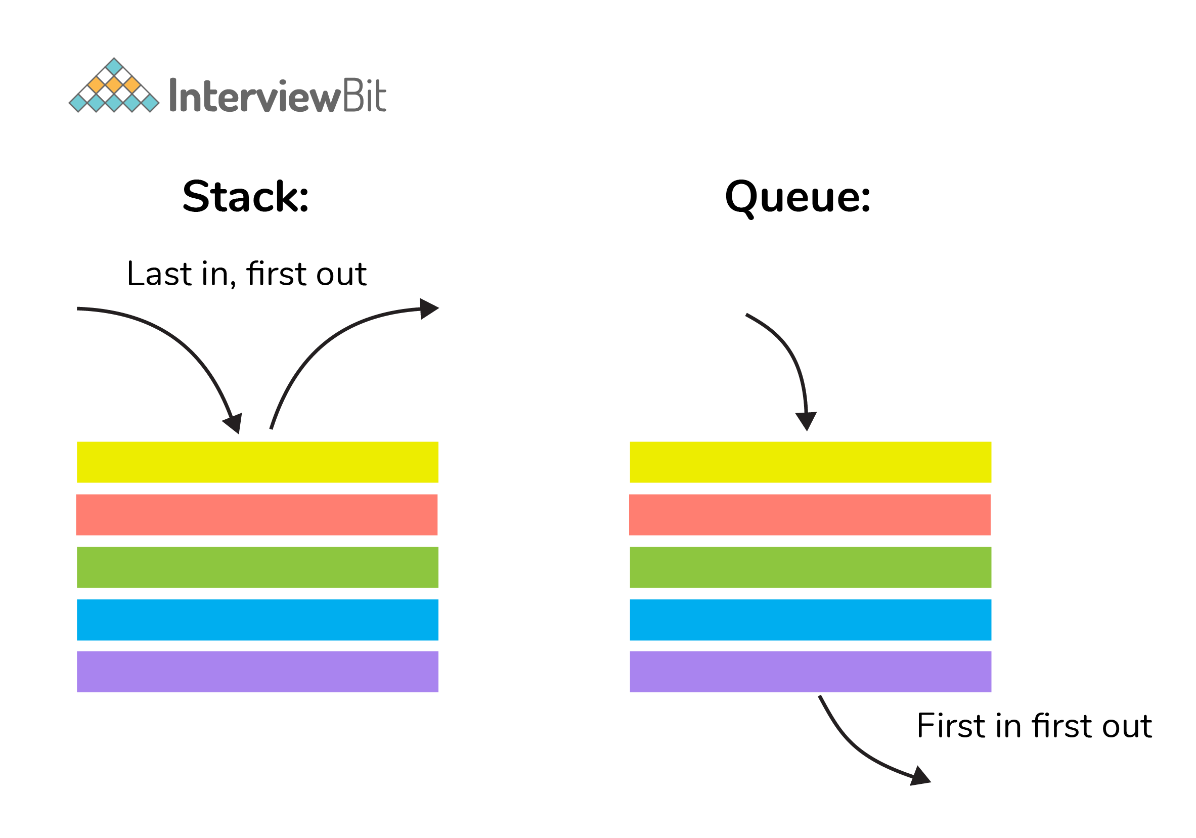
7. What is a stack data structure? What are the applications of stack?
A stack is a data structure that is used to represent the state of an application at a particular point in time. The stack consists of a series of items that are added to the top of the stack and then removed from the top. It is a linear data structure that follows a particular order in which operations are performed. LIFO (Last In First Out) or FILO (First In Last Out) are two possible orders. A stack consists of a sequence of items. The element that's added last will come out first, a real-life example might be a stack of clothes on top of each other. When we remove the cloth that was previously on top, we can say that the cloth that was added last comes out first.
Following are some applications for stack data structure:
- It acts as temporary storage during recursive operations
- Redo and Undo operations in doc editors
- Reversing a string
- Parenthesis matching
- Postfix to Infix Expressions
- Function calls order

 Real-Life Problems
 Detailed reports
8. What are different operations available in stack data structure?
Some of the main operations provided in the stack data structure are:
- push: This adds an item to the top of the stack. The overflow condition occurs if the stack is full.
- pop: This removes the top item of the stack. Underflow condition occurs if the stack is empty.
- top: This returns the top item from the stack.
- isEmpty: This returns true if the stack is empty else false.
- size: This returns the size of the stack.
9. What is a queue data structure? What are the applications of queue?
A queue is a linear data structure that allows users to store items in a list in a systematic manner. The items are added to the queue at the rear end until they are full, at which point they are removed from the queue from the front. Queues are commonly used in situations where the users want to hold items for a long period of time, such as during a checkout process. A good example of a queue is any queue of customers for a resource where the first consumer is served first.
Following are some applications of queue data structure:
- Breadth-first search algorithm in graphs
- Operating system: job scheduling operations, Disk scheduling, CPU scheduling etc.
- Call management in call centres
10. What are different operations available in queue data structure?
- enqueue: This adds an element to the rear end of the queue. Overflow conditions occur if the queue is full.
- dequeue: This removes an element from the front end of the queue. Underflow conditions occur if the queue is empty.
- isEmpty: This returns true if the queue is empty or else false.
- rear: This returns the rear end element without removing it.
- front: This returns the front-end element without removing it.
- size: This returns the size of the queue.
11. Differentiate between stack and queue data structure.
| Stack | Queue |
|---|---|
| Stack is a linear data structure where data is added and removed from the top. | Queue is a linear data structure where data is ended at the rear end and removed from the front. |
| Stack is based on LIFO(Last In First Out) principle | Queue is based on FIFO(First In First Out) principle |
| Insertion operation in Stack is known as push. | Insertion operation in Queue is known as eneque. |
| Delete operation in Stack is known as pop. | Delete operation in Queue is known as dequeue. |
| Only one pointer is available for both addition and deletion: top() | Two pointers are available for addition and deletion: front() and rear() |
| Used in solving recursion problems | Used in solving sequential processing problems |
12. How to implement a queue using stack?
A queue can be implemented using two stacks. Let q be the queue andstack1 and stack2 be the 2 stacks for implementing q. We know that stack supports push, pop, and peek operations and using these operations, we need to emulate the operations of the queue - enqueue and dequeue. Hence, queue q can be implemented in two methods (Both the methods use auxillary space complexity of O(n)):
1. By making enqueue operation costly:
- Here, the oldest element is always at the top of
stack1which ensures dequeue operation occurs in O(1) time complexity. - To place the element at top of stack1, stack2 is used.
-
Pseudocode:
- Enqueue: Here time complexity will be O(n)
enqueue(q, data):
While stack1 is not empty:
     Push everything from stack1 to stack2.
      Push data to stack1
Push everything back to stack1.- Dequeue: Here time complexity will be O(1)
deQueue(q):
 If stack1 is empty then error  else
 Pop an item from stack1 and return it
2. By making the dequeue operation costly:
- Here, for enqueue operation, the new element is pushed at the top of
stack1. Here, the enqueue operation time complexity is O(1). - In dequeue, if
stack2is empty, all elements fromstack1are moved tostack2and top ofstack2is the result. Basically, reversing the list by pushing to a stack and returning the first enqueued element. This operation of pushing all elements to a new stack takes O(n) complexity. -
Pseudocode:
- Enqueue: Time complexity: O(1)
enqueue(q, data):
Push data to stack1- Dequeue: Time complexity: O(n)
dequeue(q):
If both stacks are empty then raise error.
If stack2 is empty:
While stack1 is not empty:
 push everything from stack1 to stack2.
  Pop the element from stack2 and return it.
13. How do you implement stack using queues?
- A stack can be implemented using two queues. We know that a queue supports enqueue and dequeue operations. Using these operations, we need to develop push, pop operations.
- Let stack be ‘s’ and queues used to implement be ‘q1’ and ‘q2’. Then, stack ‘s’ can be implemented in two ways:
1. By making push operation costly:
- This method ensures that the newly entered element is always at the front of ‘q1’ so that pop operation just dequeues from ‘q1’.
- ‘q2’ is used as auxillary queue to put every new element in front of ‘q1’ while ensuring pop happens in O(1) complexity.
-
Pseudocode:
- Push element to stack s: Here push takes O(n) time complexity.
push(s, data):
    Enqueue data to q2
    Dequeue elements one by one from q1 and enqueue to q2.
    Swap the names of q1 and q2
- Pop element from stack s: Takes O(1) time complexity.
pop(s):
dequeue from q1 and return it.
2. By making pop operation costly:
- In push operation, the element is enqueued to q1.
- In pop operation, all the elements from q1 except the last remaining element, are pushed to q2 if it is empty. That last element remaining of q1 is dequeued and returned.
-
Pseudocode:
- Push element to stack s: Here push takes O(1) time complexity.
push(s,data):
Enqueue data to q1- Pop element from stack s: Takes O(n) time complexity.
pop(s):
	Step1: Dequeue every elements except the last element from q1 and enqueue to q2.
	Step2: Dequeue the last item of q1, the dequeued item is stored in result variable.
 	Step3: Swap the names of q1 and q2 (for getting updated data after dequeue)
 	Step4: Return the result.
14. What is array data structure? What are the applications of arrays?
An array data structure is a data structure that is used to store data in a way that is efficient and easy to access. It is similar to a list in that it stores data in a sequence. However, an array data structure differs from a list in that it can hold much more data than a list can. An array data structure is created by combining several arrays together. Each array is then given a unique identifier, and each array’s data is stored in the order in which they are created.
Array data structures are commonly used in databases and other computer systems to store large amounts of data efficiently. They are also useful for storing information that is frequently accessed, such as large amounts of text or images.
15. Elaborate on different types of array data structure
There are several different types of arrays:
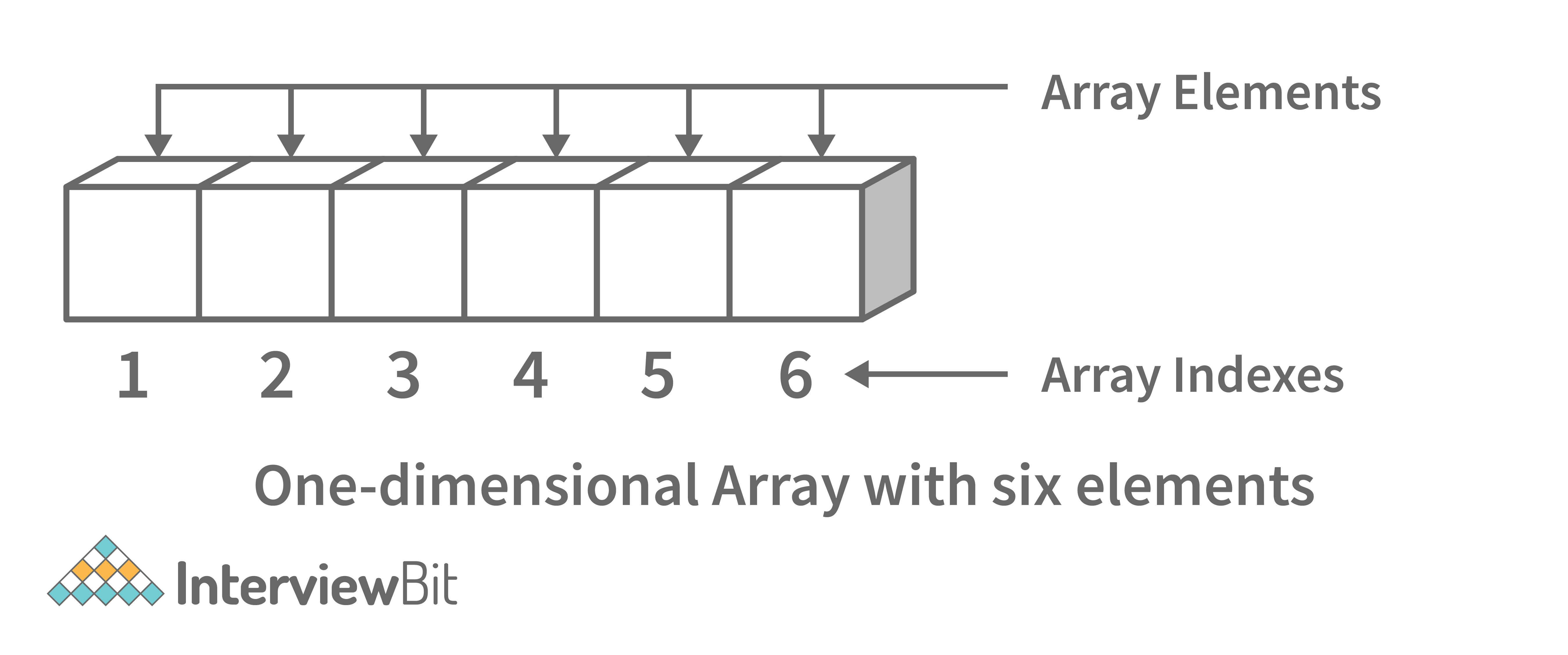
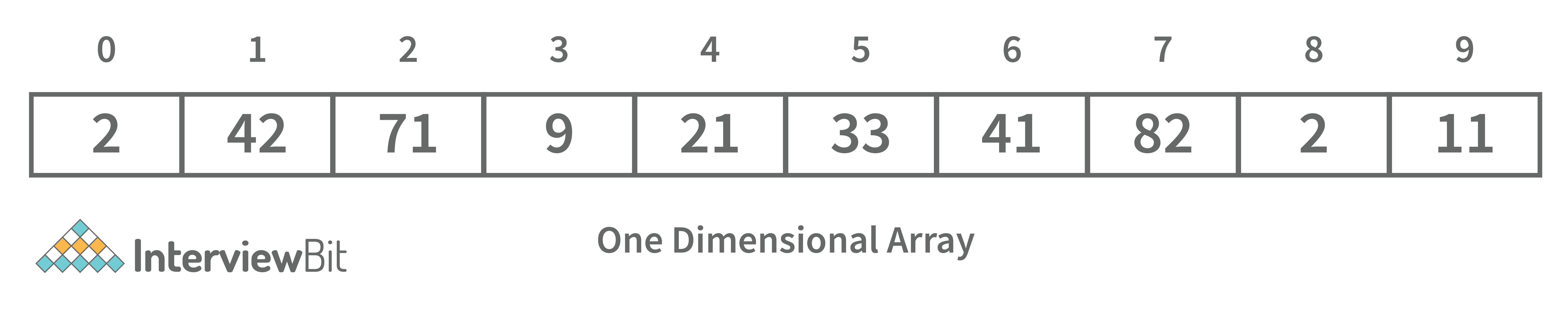
- One-dimensional array: A one-dimensional array stores its elements in contiguous memory locations, accessing them using a single index value. It is a linear data structure holding all the elements in a sequence.
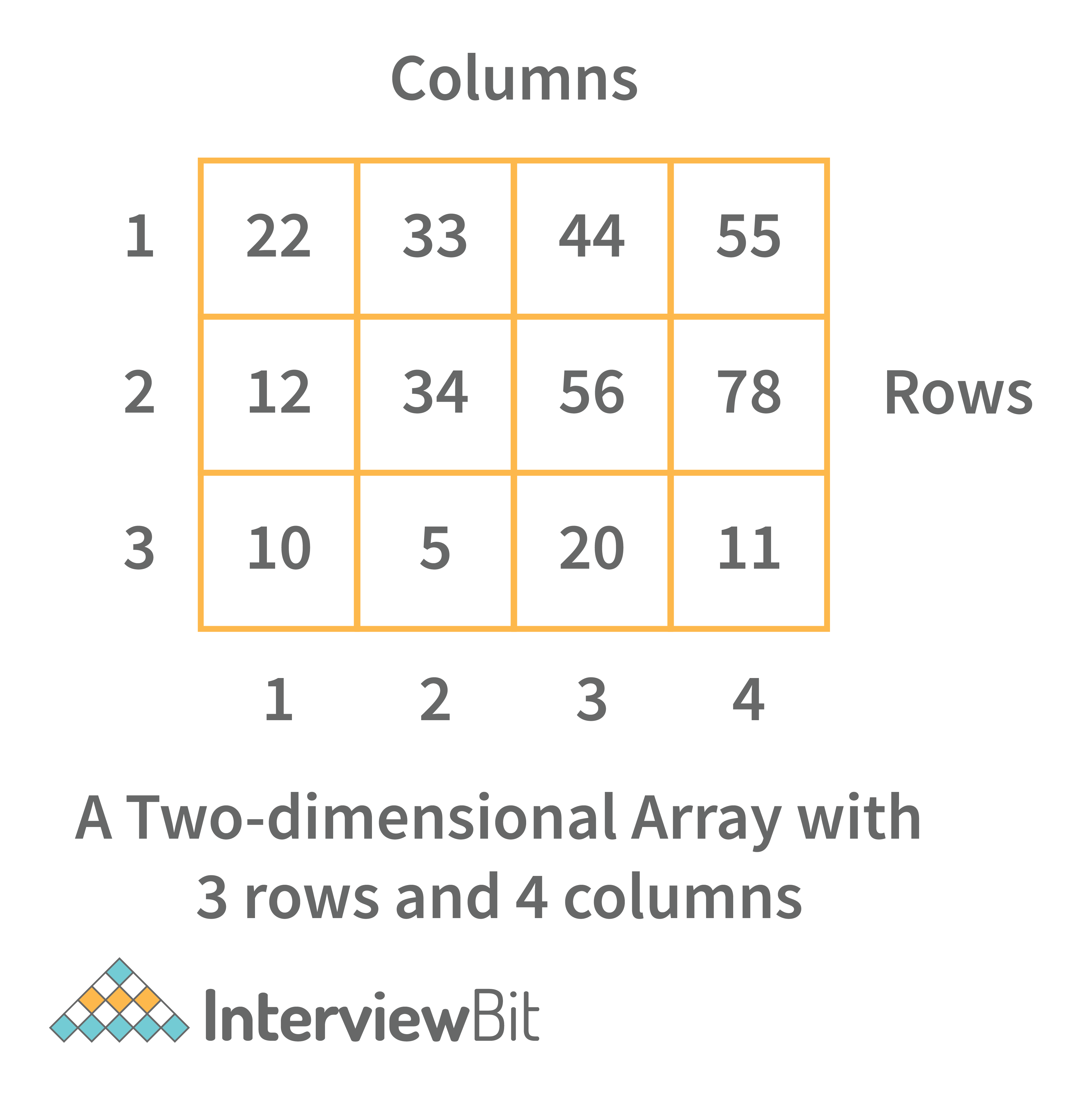
- Two-dimensional array: A two-dimensional array is a tabular array that includes rows and columns and stores data. An M × N two-dimensional array is created by grouping M rows and N columns into N columns and rows.
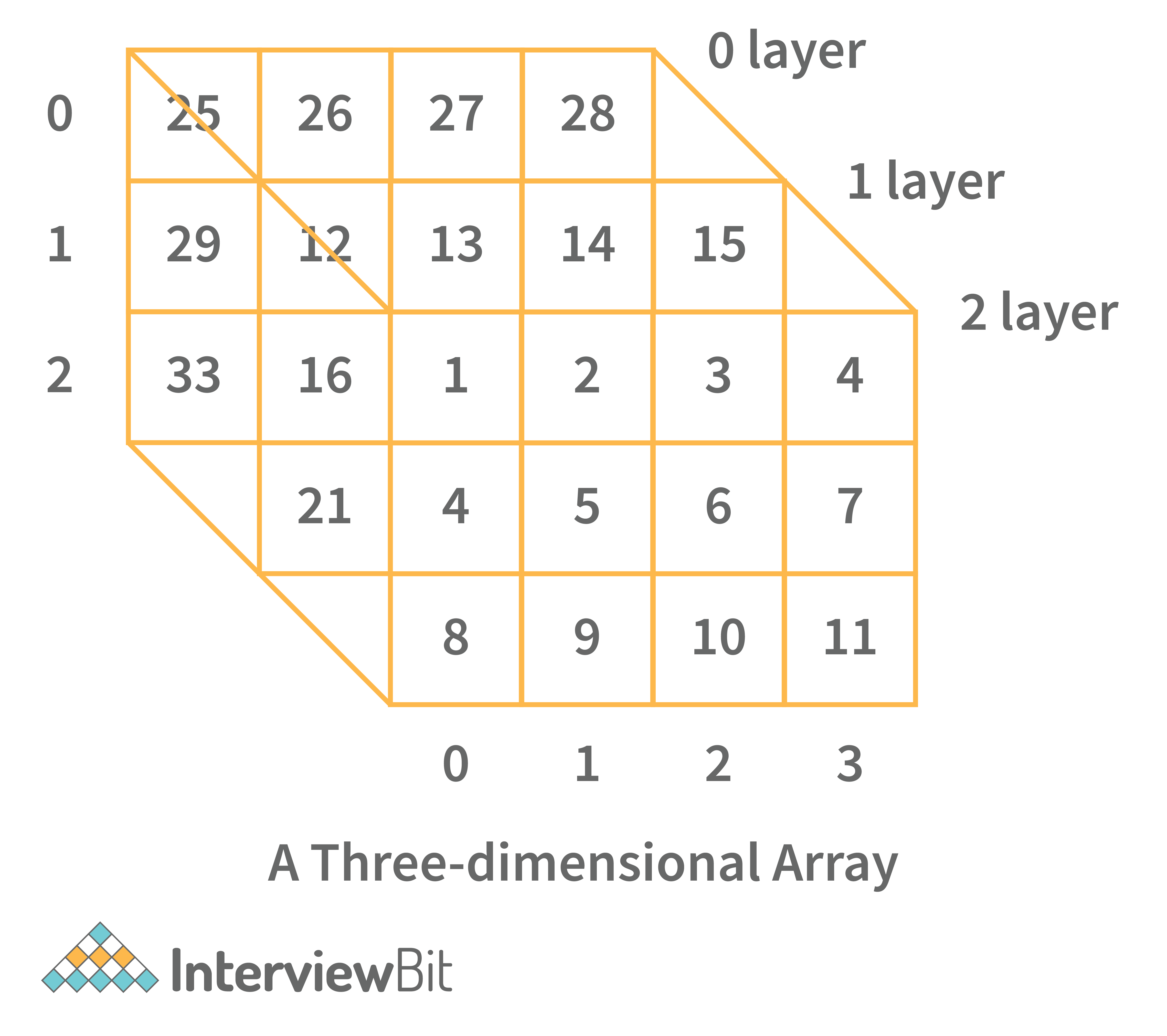
- Three-dimensional array: A three-dimensional array is a grid that has rows, columns, and depth as a third dimension. It comprises a cube with rows, columns, and depth as a third dimension. The three-dimensional array has three subscripts for a position in a particular row, column, and depth. Depth (dimension or layer) is the first index, row index is the second index, and column index is the third index.
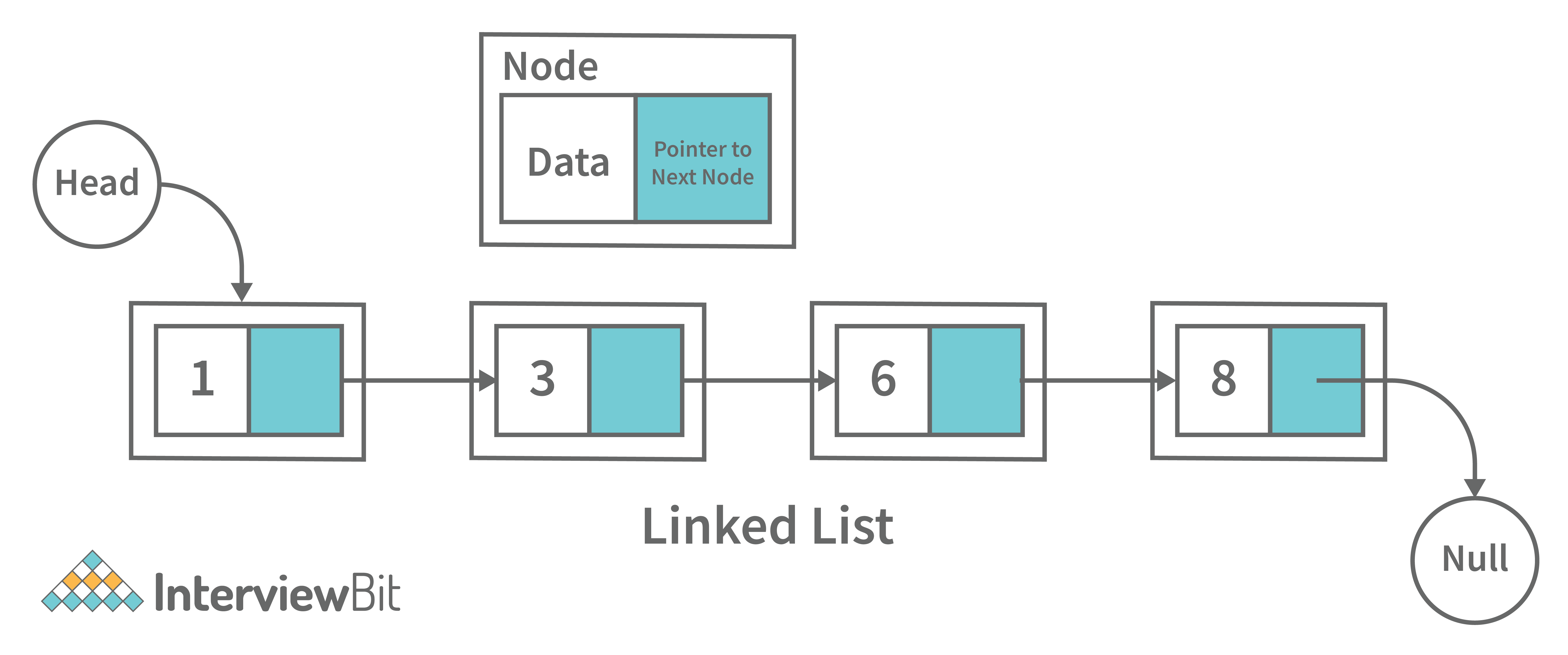
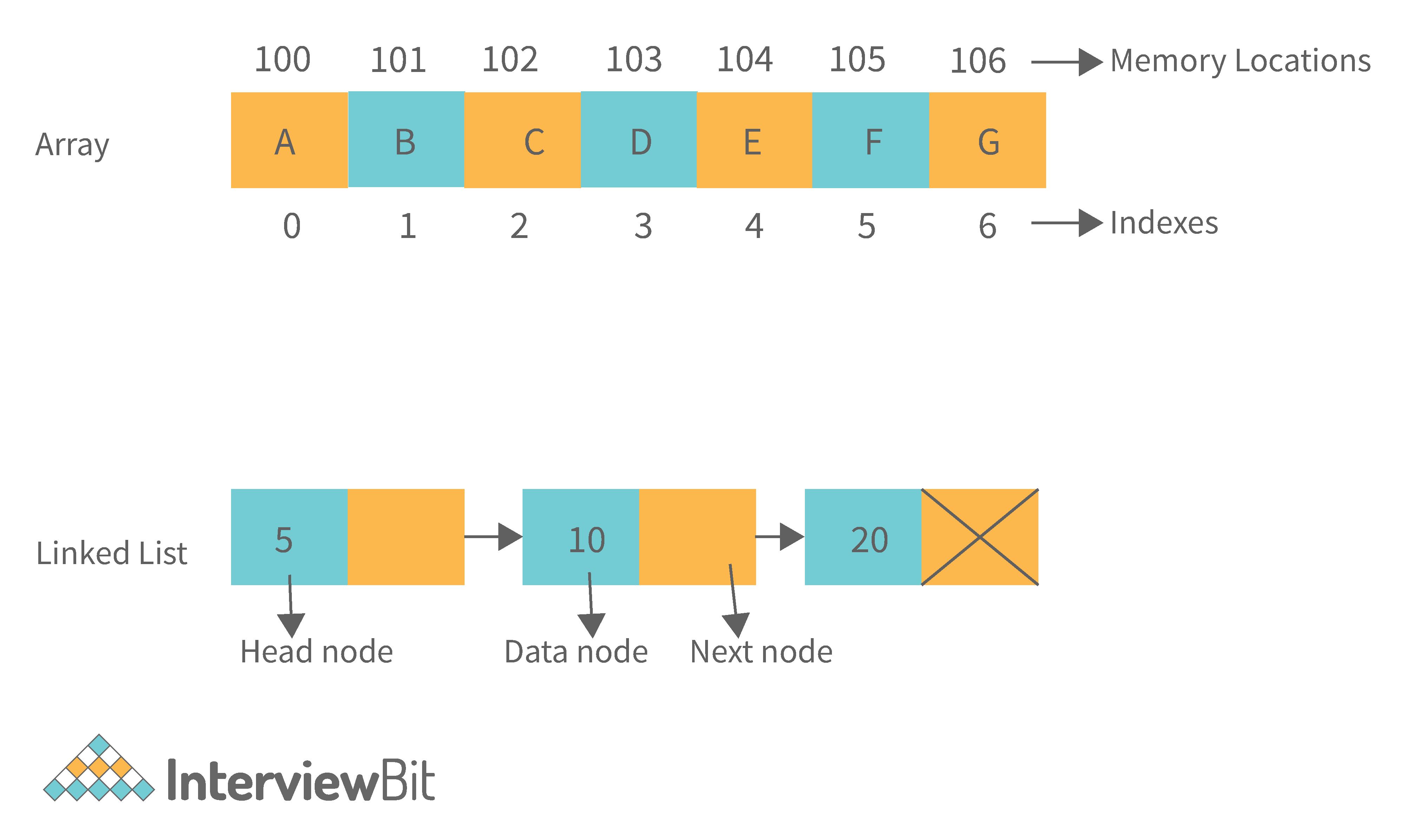
16. What is a linked list data structure? What are the applications for the Linked list?
A linked list can be thought of as a series of linked nodes (or items) that are connected by links (or paths). Each link represents an entry into the linked list, and each entry points to the next node in the sequence. The order in which nodes are added to the list is determined by the order in which they are created.
Following are some applications of linked list data structure:
- Stack, Queue, binary trees, and graphs are implemented using linked lists.
- Dynamic management for Operating System memory.
- Round robin scheduling for operating system tasks.
- Forward and backward operation in the browser.
17. Elaborate on different types of Linked List data structures?
Following are different types of linked lists:
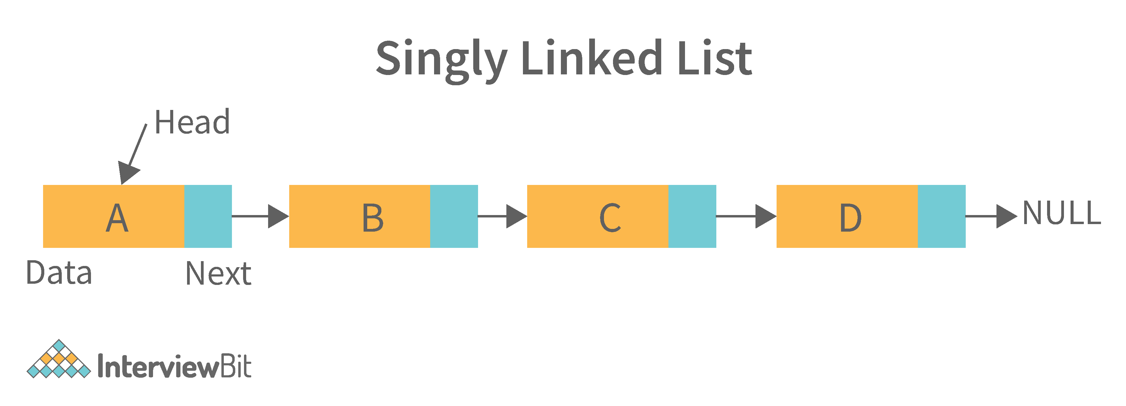
1. Singly Linked List: A singly linked list is a data structure that is used to store multiple items. The items are linked together using the key. The key is used to identify the item and is usually a unique identifier. In a singly linked list, each item is stored in a separate node. The node can be a single object or it can be a collection of objects. When an item is added to the list, the node is updated and the new item is added to the end of the list. When an item is removed from the list, the node that contains the removed item is deleted and its place is taken by another node. The key of a singly linked list can be any type of data structure that can be used to identify an object. For example, it could be an integer, a string, or even another singly linked list. Singly-linked lists are useful for storing many different types of data. For example, they are commonly used to store lists of items such as grocery lists or patient records. They are also useful for storing data that is time sensitive such as stock market prices or flight schedules.
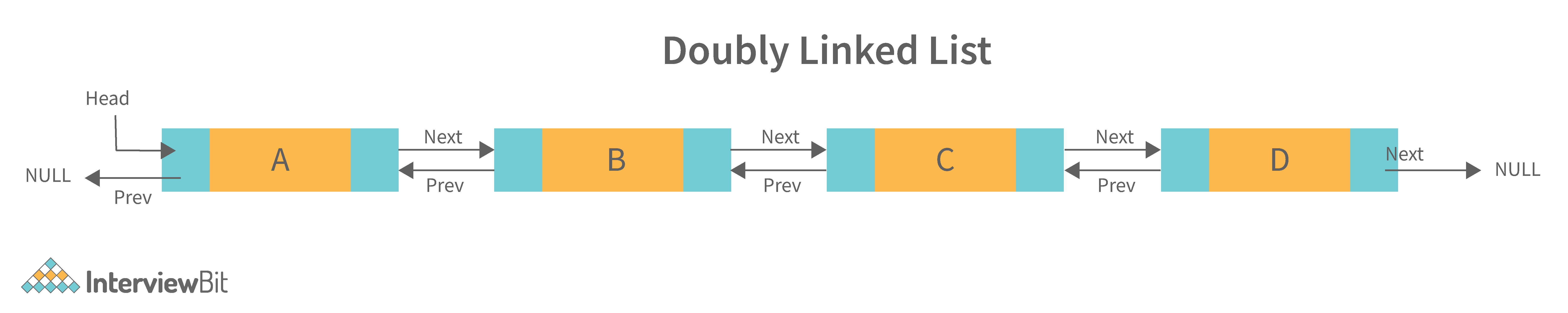
2. Doubly Linked List: A doubly linked list is a data structure that allows for two-way data access such that each node in the list points to the next node in the list and also points back to its previous node. In a doubly linked list, each node can be accessed by its address, and the contents of the node can be accessed by its index. It's ideal for applications that need to access large amounts of data in a fast manner. A disadvantage of a doubly linked list is that it is more difficult to maintain than a single-linked list. In addition, it is more difficult to add and remove nodes than in a single-linked list.
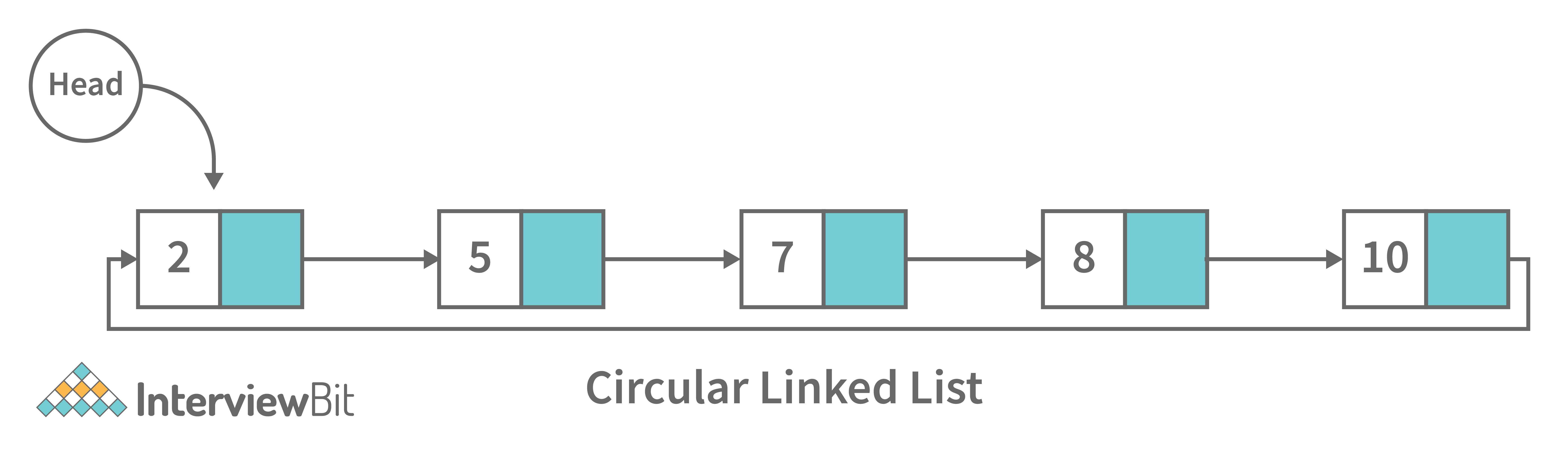
3. Circular Linked List: A circular linked list is a unidirectional linked list where each node points to its next node and the last node points back to the first node, which makes it circular.
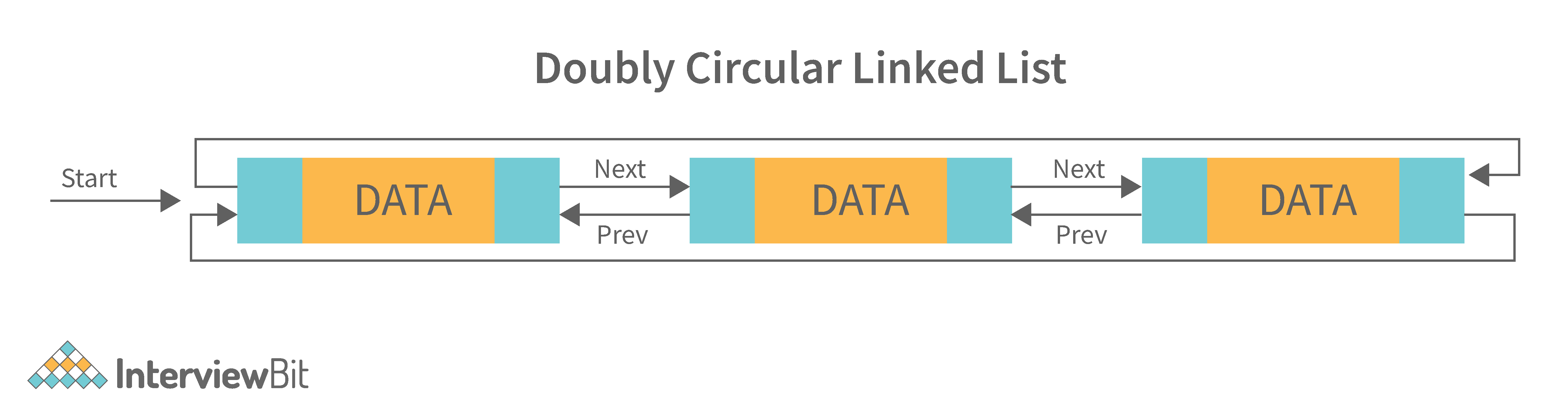
4. Doubly Circular Linked List: A doubly circular linked list is a linked list where each node points to its next node and its previous node and the last node points back to the first node and first node’s previous points to the last node.
5. Header List: A list that contains the header node at the beginning of the list, is called the header-linked list. This is helpful in calculating some repetitive operations like the number of elements in the list etc.
18. Difference between Array and Linked List.
| Arrays | Linked Lists |
|---|---|
| An array is a collection of data elements of the same type. | A linked list is a collection of entities known as nodes. The node is divided into two sections: data and address. |
| It keeps the data elements in a single memory. | It stores elements at random, or anywhere in the memory. |
| The memory size of an array is fixed and cannot be changed during runtime. | The memory size of a linked list is allocated during runtime. |
| An array's elements are not dependent on one another. | Linked List elements are dependent on one another. |
| It is easier and faster to access an element in an array. | In the linked list, it takes time to access an element. |
| Memory utilization is ineffective in the case of an array. | Memory utilization is effective in the case of linked lists. |
| Operations like insertion and deletion take longer time in an array. | Operations like insertion and deletion are faster in the linked list. |
19. What is an asymptotic analysis of an algorithm?
Asymptotic analysis of an algorithm defines the run-time performance as per its mathematical boundations. Asymptotic analysis helps us articulate the best case(Omega Notation, Ω), average case(Theta Notation, θ), and worst case(Big Oh Notation, Ο) performance of an algorithm.
20. What is hashmap in data structure?
Hashmap is a data structure that uses an implementation of a hash table data structure which allows access to data in constant time (O(1)) complexity if you have the key.
21. What is the requirement for an object to be used as key or value in HashMap?
- The key or value object that gets used in the hashmap must implement
equals()andhashcode()method. - The hash code is used when inserting the key object into the map and the equals method is used when trying to retrieve a value from the map.
22. How does HashMap handle collisions in Java?
- The
java.util.HashMapclass in Java uses the approach of chaining to handle collisions. In chaining, if the new values with the same key are attempted to be pushed, then these values are stored in a linked list stored in a bucket of the key as a chain along with the existing value. - In the worst-case scenario, it can happen that all keys might have the same hashcode, which will result in the hash table turning into a linked list. In this case, searching a value will take O(n) complexity as opposed to O(1) time due to the nature of the linked list. Hence, care has to be taken while selecting hashing algorithm.
23. What is the time complexity of basic operations get() and put() in HashMap class?
The time complexity is O(1) assuming that the hash function used in the hash map distributes elements uniformly among the buckets.
Data Structure Interview Questions for Experienced
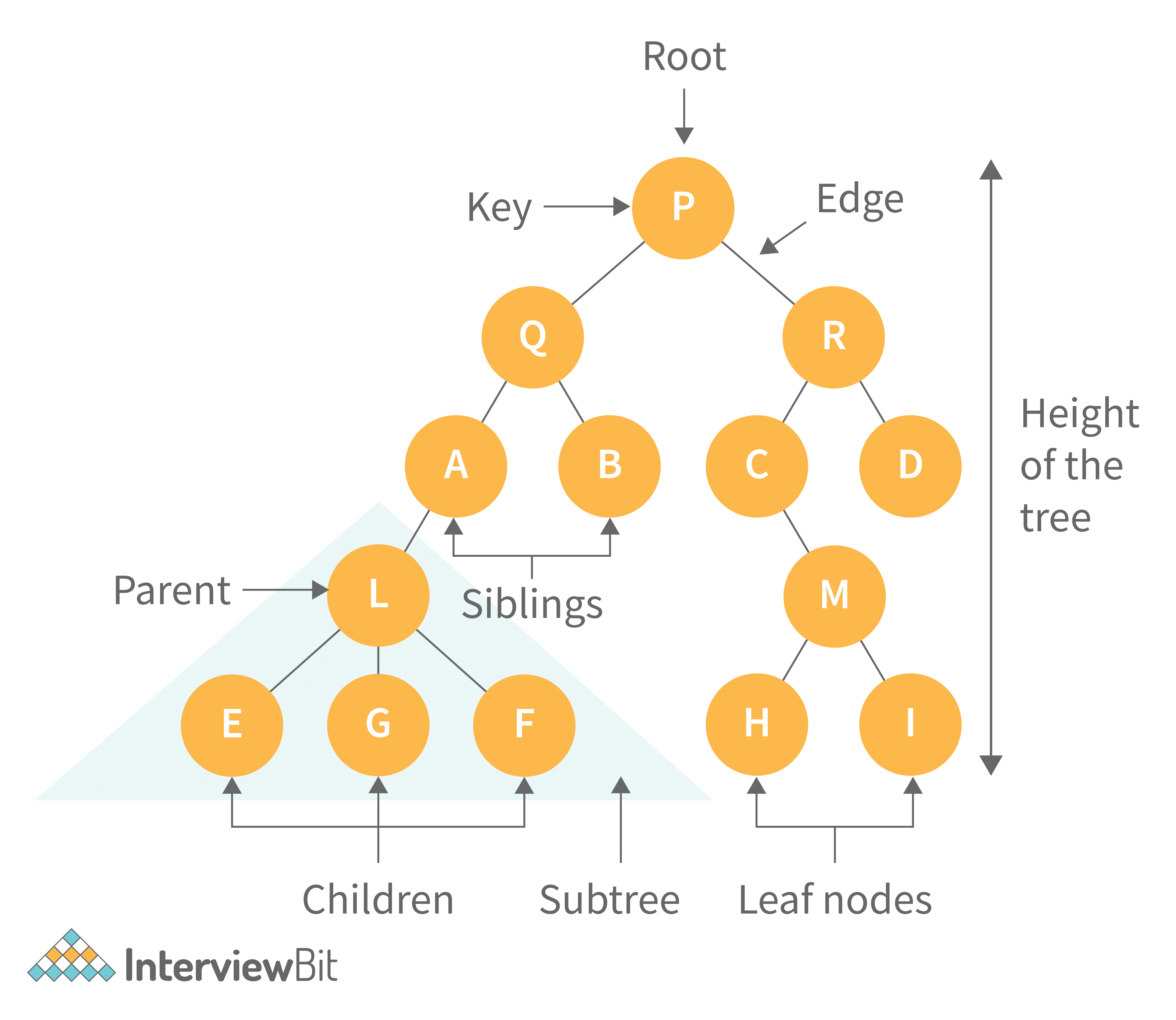
1. What is binary tree data structure? What are the applications for binary trees?
A binary tree is a data structure that is used to organize data in a way that allows for efficient retrieval and manipulation. It is a data structure that uses two nodes, called leaves and nodes, to represent the data. The leaves represent the data and the nodes represent the relationships between the leaves. Each node has two children, called siblings, and each child has one parent. The parent is the node that is closest to the root of the tree. When a node is deleted from the tree, it is deleted from both its child and its parent.
Following are some applications for binary tree data structure:
- It's widely used in computer networks for storing routing table information.
- Decision Trees.
- Expression Evaluation.
- Database indices.
2. What is binary search tree data structure? What are the applications for binary search trees?
A binary search tree is a data structure that stores items in sorted order. In a binary search tree, each node stores a key and a value. The key is used to access the item and the value is used to determine whether the item is present or not. The key can be any type of value such as an integer, floating point number, character string, or even a combination of these types. The value can be any type of items such as an integer, floating point number, character string, or even a combination of these types. When a node is added to the tree, its key is used to access the item stored at that node. When a node is removed from the tree, its key is used to access the item stored at that node.
A binary search tree is a special type of binary tree that has a specific order of elements in it. It has three basic qualities:
- All elements in the left subtree of a node should have a value less than or equal to the parent node's value, and
- All elements in the right subtree of a node should have a value greater than or equal to the parent node's value.
- Both the left and right subtrees must be binary search trees too.
Following are some applications for binary tree data structure:
- It is used for indexing and multi-level indexing.
- It is used for implementing various search algorithms.
- It is helpful in organizing a sorted stream of data.
3. What are tree traversals?
Tree traversal is the process of visiting all the nodes of a tree. Since the root (head) is the first node and all nodes are connected via edges (or links) we always start with that node. There are three ways which we use to traverse a tree −
1. Inorder Traversal:
- Algorithm:
- Step 1. Traverse the left subtree, i.e., call Inorder(root.left)
- Step 2. Visit the root.
- Step 3. Traverse the right subtree, i.e., call Inorder(root.right)
- Inorder traversal in Java:
     // Print inorder traversal of given tree.
     void printInorderTraversal(Node root)
     {
         if (root == null)
             return;
         //first traverse to the left subtree
         printInorderTraversal(root.left);
         //then print the data of node
         System.out.print(root.data + " ");
         //then traverse to the right subtree
         printInorderTraversal(root.right);
}- Uses: In binary search trees (BST), inorder traversal gives nodes in ascending order.
2. Preorder Traversal:
- Algorithm:
- Step 1. Visit the root.
- Step 2. Traverse the left subtree, i.e., call Preorder(root.left)
- Step 3. Traverse the right subtree, i.e., call Preorder(root.right)
- Preorder traversal in Java:
 // Print preorder traversal of given tree.
    void printPreorderTraversal(Node root)
    {
        if (root == null)
            return;
        //first print the data of node
        System.out.print(root.data + " ");
        //then traverse to the left subtree
        printPreorderTraversal(root.left);
        //then traverse to the right subtree
        printPreorderTraversal(root.right);
}- Uses:
- Preorder traversal is commonly used to create a copy of the tree.
- It is also used to get prefix expression of an expression tree.
3. Postorder Traversal:
- Algorithm:
- Step 1. Traverse the left subtree, i.e., call Postorder(root.left)
- Step 2. Traverse the right subtree, i.e., call Postorder(root.right)
- Step 3. Visit the root.
- Postorder traversal in Java:
// Print postorder traversal of given tree.
void printPostorderTraversal(Node root)
{
 if (root == null)
     return;
 //first traverse to the left subtree
 printPostorderTraversal(root.left);
 //then traverse to the right subtree
 printPostorderTraversal(root.right);
 //then print the data of node
 System.out.print(root.data + " ");
}- Uses:
- Postorder traversal is commonly used to delete the tree.
- It is also useful to get the postfix expression of an expression tree.
Consider the following tree as an example, then:
- Inorder Traversal => Left, Root, Right : [4, 2, 5, 1, 3]
- Preorder Traversal => Root, Left, Right : [1, 2, 4, 5, 3]
- Postorder Traversal => Left, Right, Root : [4, 5, 2, 3, 1]
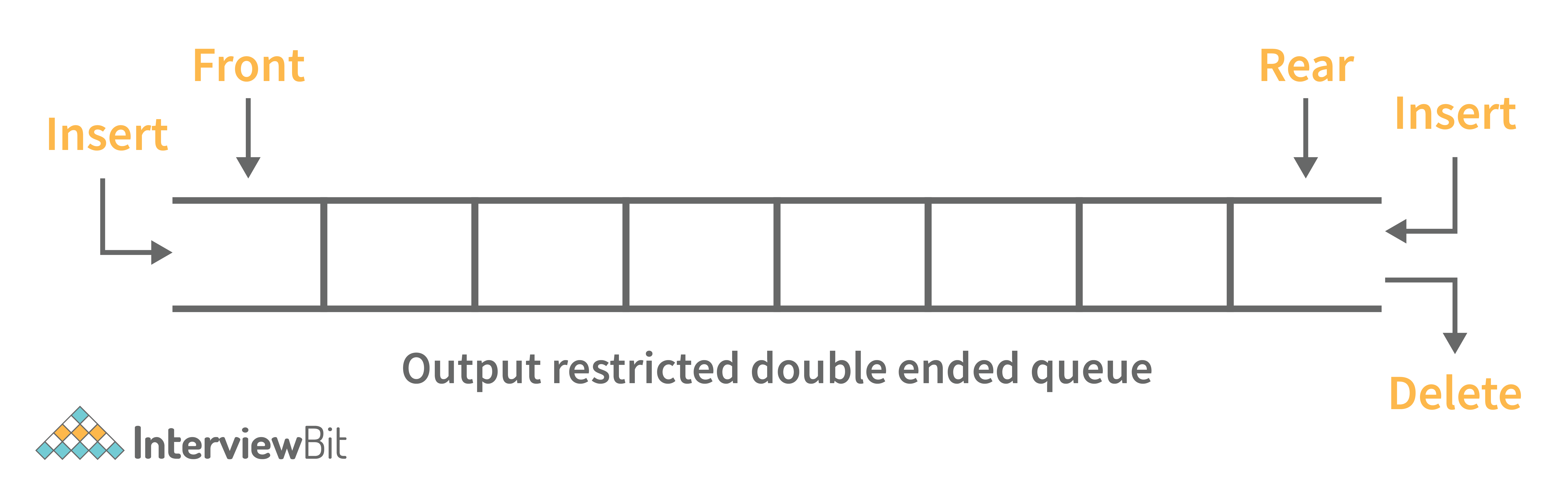
4. What is a deque data structure and its types? What are the applications for deque?
A deque can be thought of as an array of items, but with one important difference: Instead of pushing and popping items off the end to make room, deques are designed to allow items to be inserted at either end. This property makes deques well-suited for performing tasks such as keeping track of inventory, scheduling tasks, or handling large amounts of data.
There are two types of deque:
- Input Restricted Deque: Insertion operations are performed at only one end while deletion is performed at both ends in the input restricted queue.
- Output Restricted Deque: Deletion operations are performed at only one end while insertion is performed at both ends in the output restricted queue.
Following are some real-time applications for deque data structure:
- It can be used as both stack and queue, as it supports all the operations for both data structures.
- Web browser’s history can be stored in a deque.
- Operating systems job scheduling algorithm.
5. What are some key operations performed on the Deque data structure?
Following are the key operations available deque:
- insertFront(): This adds an element to the front of the Deque.
- insertLast(): This adds an element to the rear of the Deque.
- deleteFront(): This deletes an element from the front of the Deque.
- deleteLast():This deletes an element from the front of the Deque.
- getFront(): This gets an element from the front of the Deque.
- getRear(): This gets an element from the rear of the Deque.
- isEmpty(): This checks whether Deque is empty or not.
- isFull(): This checks whether Deque is full or not.
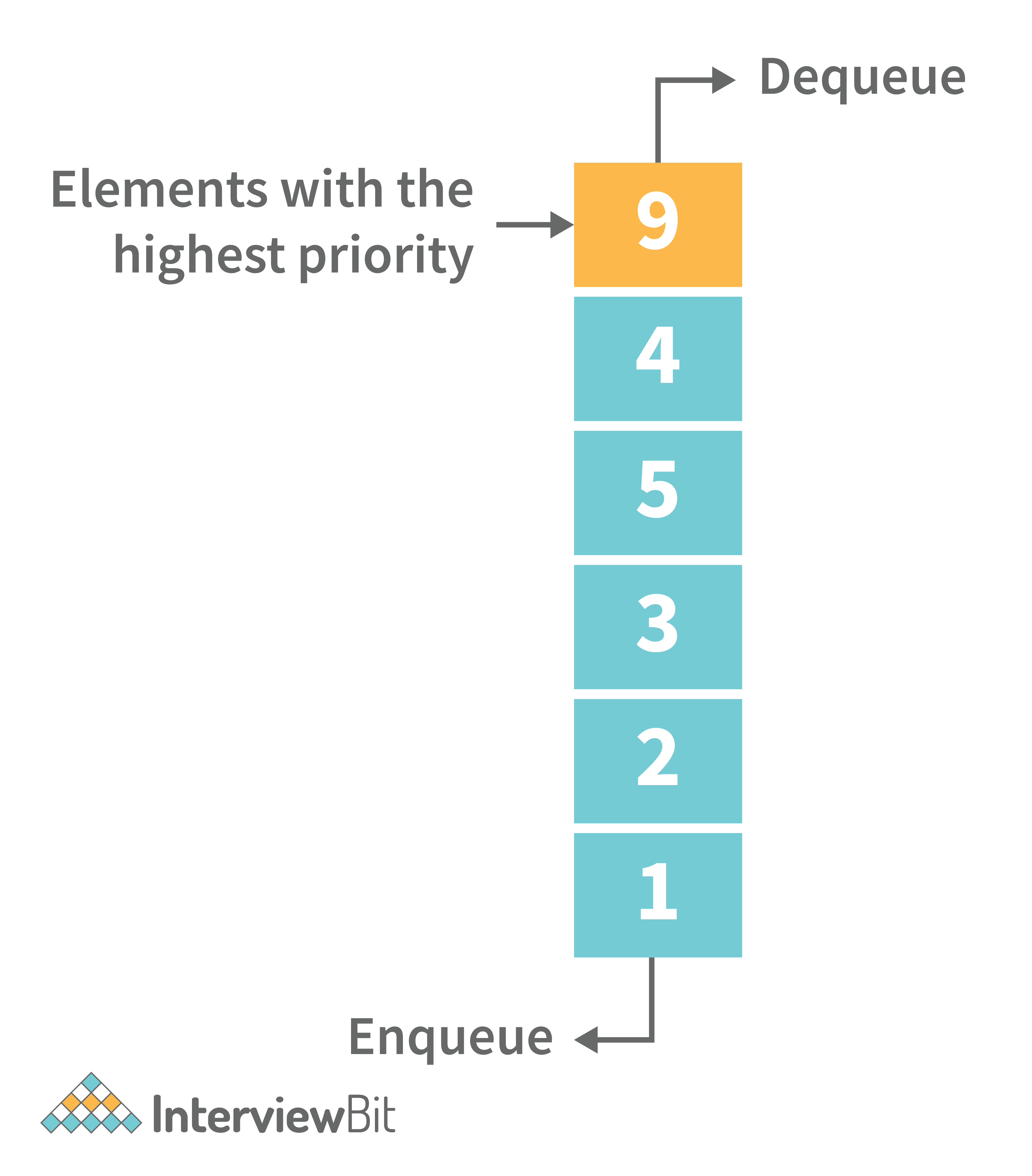
6. What is a priority queue? What are the applications for priority queue?
Priority Queue is an abstract data type that is similar to a queue in that each element is assigned a priority value. The order in which elements in a priority queue are served is determined by their priority (i.e., the order in which they are removed). If the elements have the same priority, they are served in the order they appear in the queue.
Following are some real-time applications for priority queue:
- Used in graph algorithms like Dijkstra, Prim’s Minimum spanning tree etc.
- Huffman code for data compression
- Finding Kth Largest/Smallest element
7. Compare different implementations of priority queue
The following table contains an asymptotic analysis of different implementations of a priority queue:
| Operations | peek | insert | delete |
|---|---|---|---|
| Linked List | O(1) | O(n) | O(1) |
| Binary Heap | O(1) | O(log n) | O(log n) |
| Binary Search Tree | O(1) | O(log n) | O(log n) |
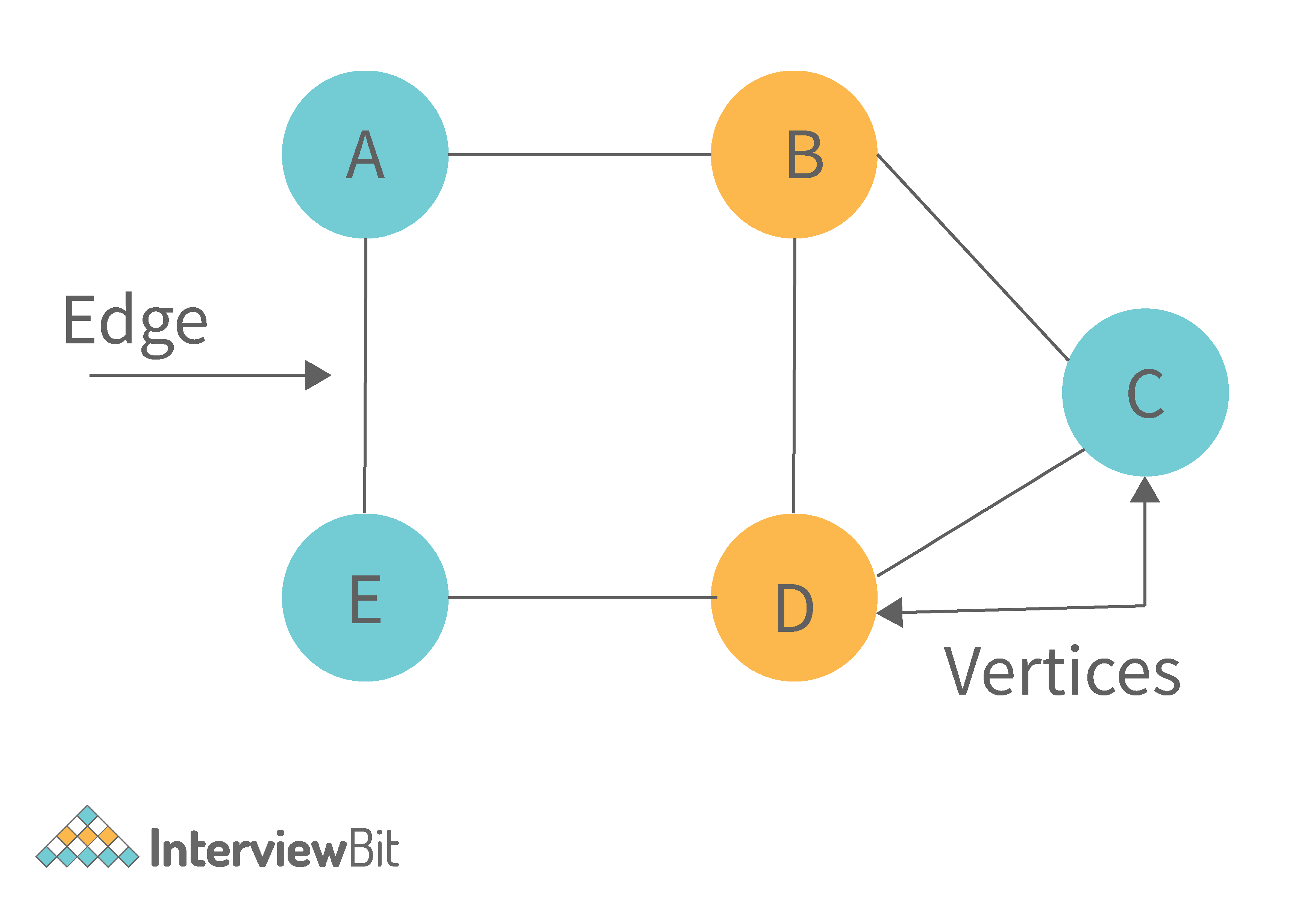
8. What is graph data structure and its representations? What are the applications for graphs?
A graph is a type of non-linear data structure made up of nodes and edges. The nodes are also known as vertices, and edges are lines or arcs that connect any two nodes in the graph.
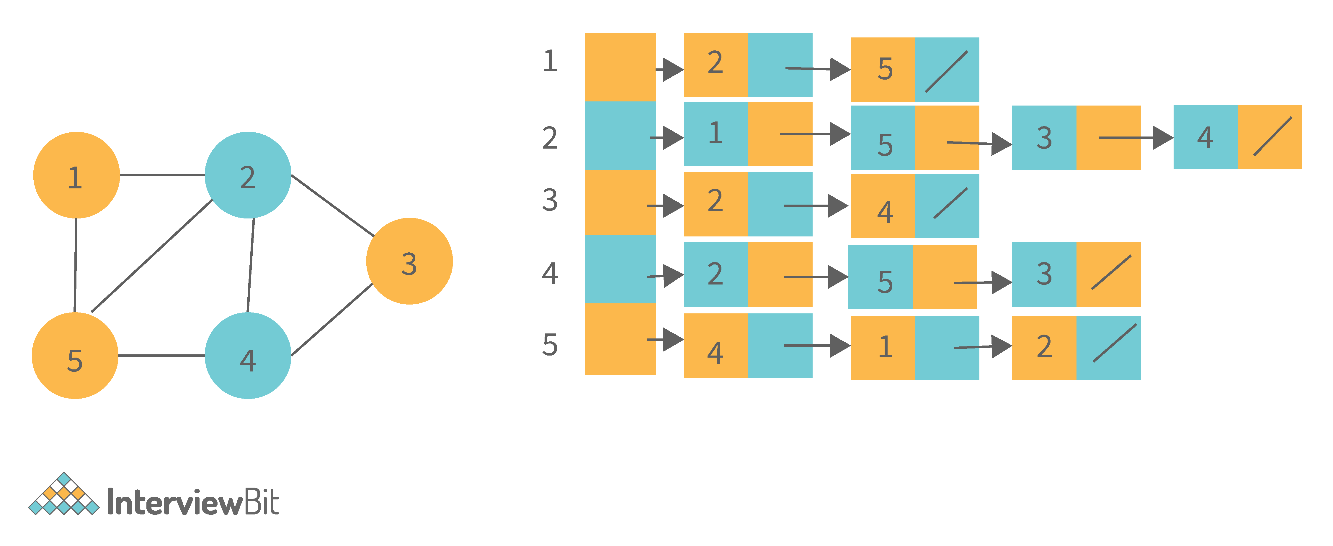
The following are the two most common graph representations:
1. Adjacency Matrix: Adjacency Matrix is a two-dimensional array with the dimensions V x V, where V is the number of vertices in a graph. Representation is simpler to implement and adhere to. It takes O(1) time to remove an edge. Queries such as whether there is an edge from vertex 'u' to vertex 'v' are efficient and can be completed in O(1).
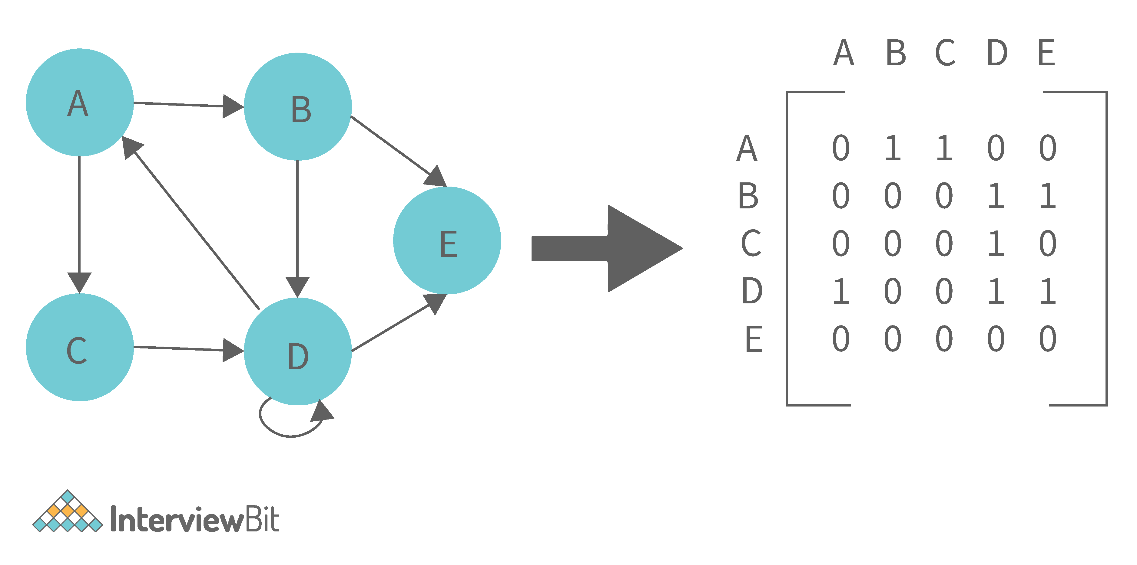
One of the cons of this representation is that even if the graph is sparse (has fewer edges), it takes up the same amount of space. Adding a vertex takes O(V^2). It also takes O(V) time to compute all of a vertex's neighbours, which is not very efficient.
2. Adjacency List: In this method, each Node holds a list of Nodes that are directly connected to that vertex. Each node at the end of the list is connected with null values to indicate that it is the last node in the list. This saves space O(|V|+|E|). In the worst-case scenario, a graph can have C(V, 2) edges, consuming O(V^2) space. It is simpler to add a vertex. It takes the least amount of time to compute all of a vertex's neighbours.
One of the cons of this representation is that queries such as "is there an edge from vertex u to vertex v?" are inefficient and take O (V) in the worst case.
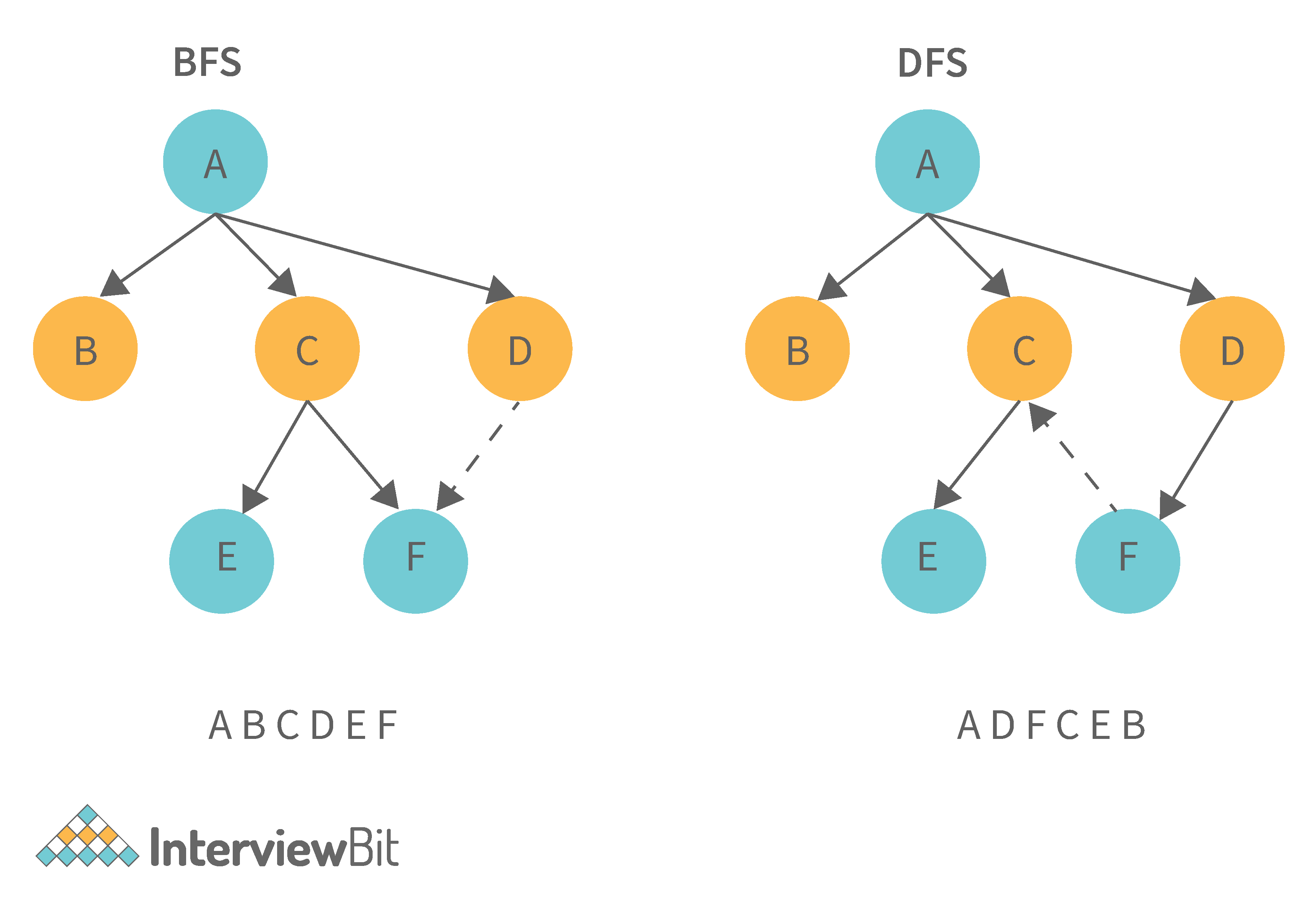
9. What is the difference between the Breadth First Search (BFS) and Depth First Search (DFS)?
| Breadth First Search (BFS) | Depth First Search (DFS) |
|---|---|
| It stands for “Breadth First Search” | It stands for “Depth First Search” |
| BFS (Breadth First Search) finds the shortest path using the Queue data structure. | DFS (Depth First Search) finds the shortest path using the Stack data structure. |
| We walk through all nodes on the same level before passing to the next level in BFS. | DFS begins at the root node and proceeds as far as possible through the nodes until we reach the node with no unvisited nearby nodes. |
| When compared to DFS, BFS is slower. | When compared to BFS, DFS is faster. |
| BFS performs better when the target is close to the source. | DFS performs better when the target is far from the source. |
| BFS necessitates more memory. | DFS necessitates less memory. |
| Nodes that have been traversed multiple times are removed from the queue. | When there are no more nodes to visit, the visited nodes are added to the stack and then removed. |
| Backtracking is not an option in BFS. | The DFS algorithm is a recursive algorithm that employs the concept of backtracking. |
| It is based on the FIFO principle (First In First Out). | It is based on the LIFO principle (Last In First Out). |
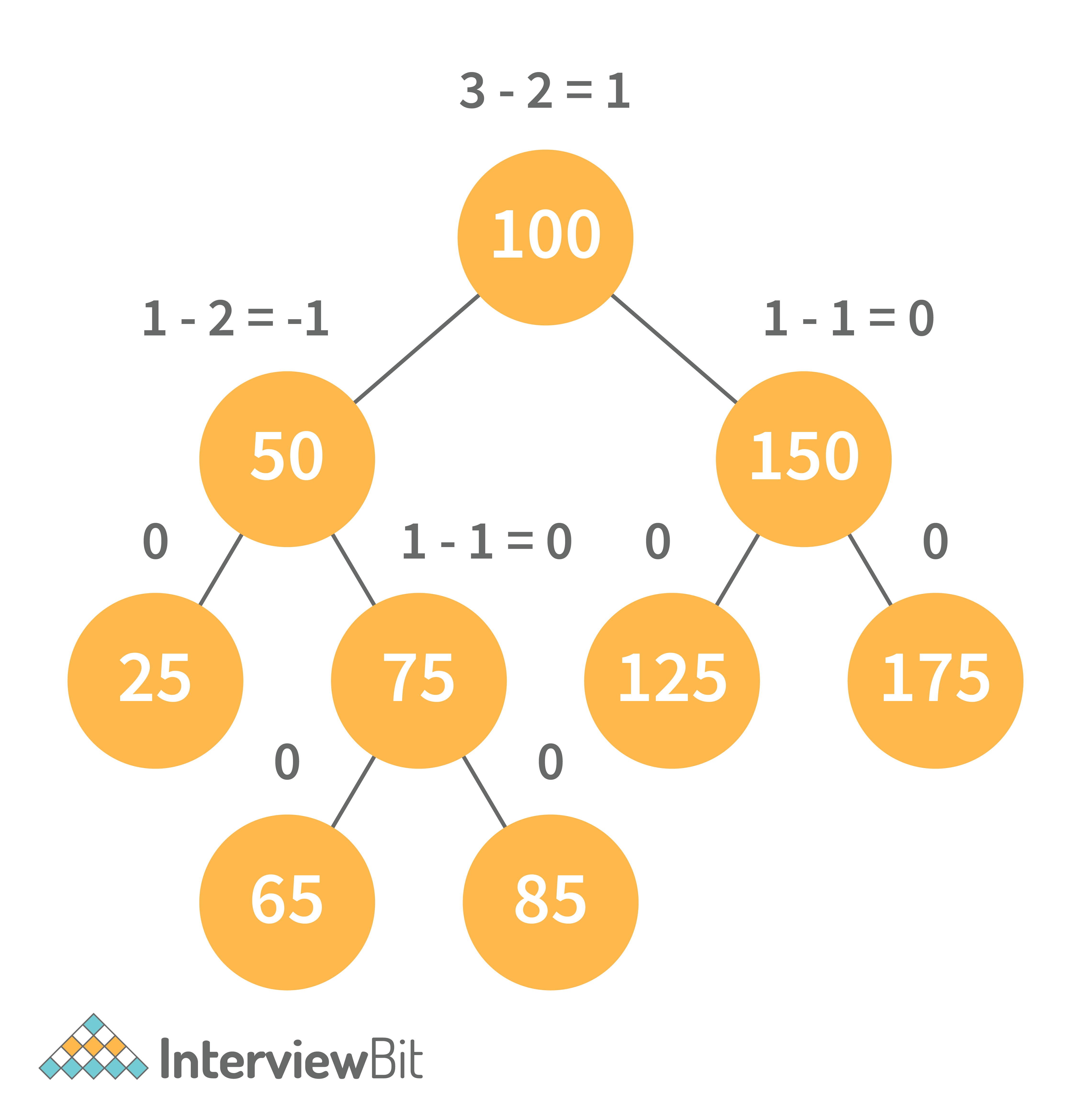
10. What is AVL tree data structure, its operations, and its rotations? What are the applications for AVL trees?
AVL trees are height balancing binary search trees named after their inventors Adelson, Velski, and Landis. The AVL tree compares the heights of the left and right subtrees and ensures that the difference is less than one. This distinction is known as the Balance Factor.
BalanceFactor = height(left-subtree) − height(right-subtree)
We can perform the following two operations on AVL tree:
- Insertion: Insertion in an AVL tree is done in the same way that it is done in a binary search tree. However, it may cause a violation in the AVL tree property, requiring the tree to be balanced. Rotations can be used to balance the tree.
- Deletion: Deletion can also be performed in the same manner as in a binary search tree. Because deletion can disrupt the tree's balance, various types of rotations are used to rebalance it.
An AVL tree can balance itself by performing the four rotations listed below:
- Left rotation: When a node is inserted into the right subtree of the right subtree and the tree becomes unbalanced, we perform a single left rotation.
- Right rotation: If a node is inserted in the left subtree of the left subtree, the AVL tree may become unbalanced. The tree then requires right rotation.
- Left-Right rotation: The RR rotation is performed first on the subtree, followed by the LL rotation on the entire tree.
- Right-Left rotation: The LL rotation is performed first on the subtree, followed by the RR rotation on the entire tree.
Following are some real-time applications for AVL tree data structure:
- AVL trees are typically used for in-memory sets and dictionaries.
- AVL trees are also widely used in database applications where there are fewer insertions and deletions but frequent data lookups are required.
- Apart from database applications, it is used in applications that require improved searching.
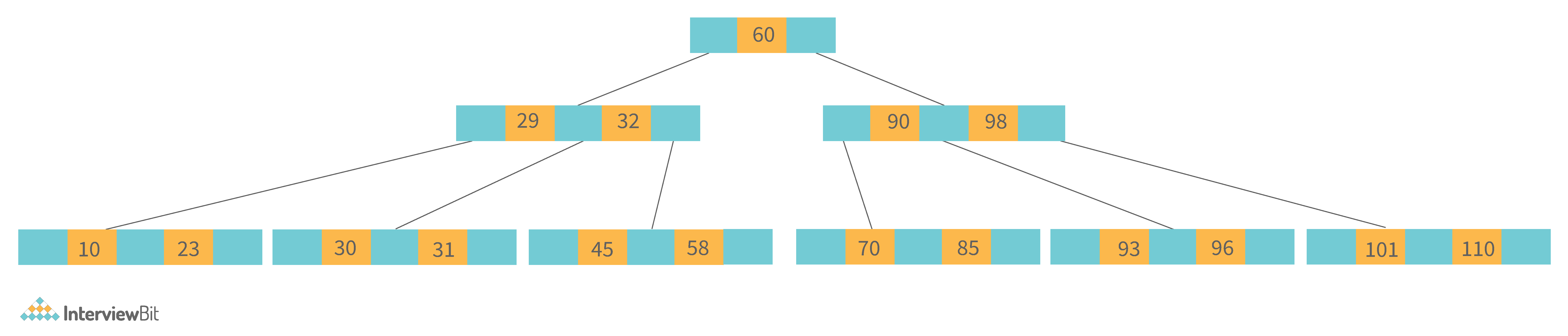
11. What is a B-tree data structure? What are the applications for B-trees?
The B Tree is a type of m-way tree that is commonly used for disc access. A B-Tree with order m can only have m-1 keys and m children. One of the primary reasons for using a B tree is its ability to store a large number of keys in a single node as well as large key values while keeping the tree's height relatively small.
A B-tree of order 4 is shown below in the image:
Following are the key properties of a B-tree data structure:
- All of the leaves are at the same height.
- The term minimum degree 't' describes a B-Tree. The value of t is determined by the size of the disc block.
- Except for root, every node must have at least t-1 keys. The root must contain at least one key.
- All nodes (including root) can have no more than 2*t - 1 keys.
- The number of children of a node is equal to its key count plus one.
- A node's keys are sorted in ascending order. The child of two keys k1 and k2 contains all keys between k1 and k2.
- In contrast to Binary Search Tree, B-Tree grows and shrinks from the root.
Following are real-time applications of a B-Tree data structure:
- It is used to access data stored on discs in large databases.
- Using a B tree, you can search for data in a data set in significantly less time.
- The indexing feature allows for multilevel indexing.
- The B-tree approach is also used by the majority of servers.
12. Define Segment Tree data structure and its applications.
A segment Tree is a binary tree that is used to store intervals or segments. The Segment Tree is made up of nodes that represent intervals. Segment Tree is used when there are multiple range queries on an array and changes to array elements.
The segment tree of array A[7] will look like this:
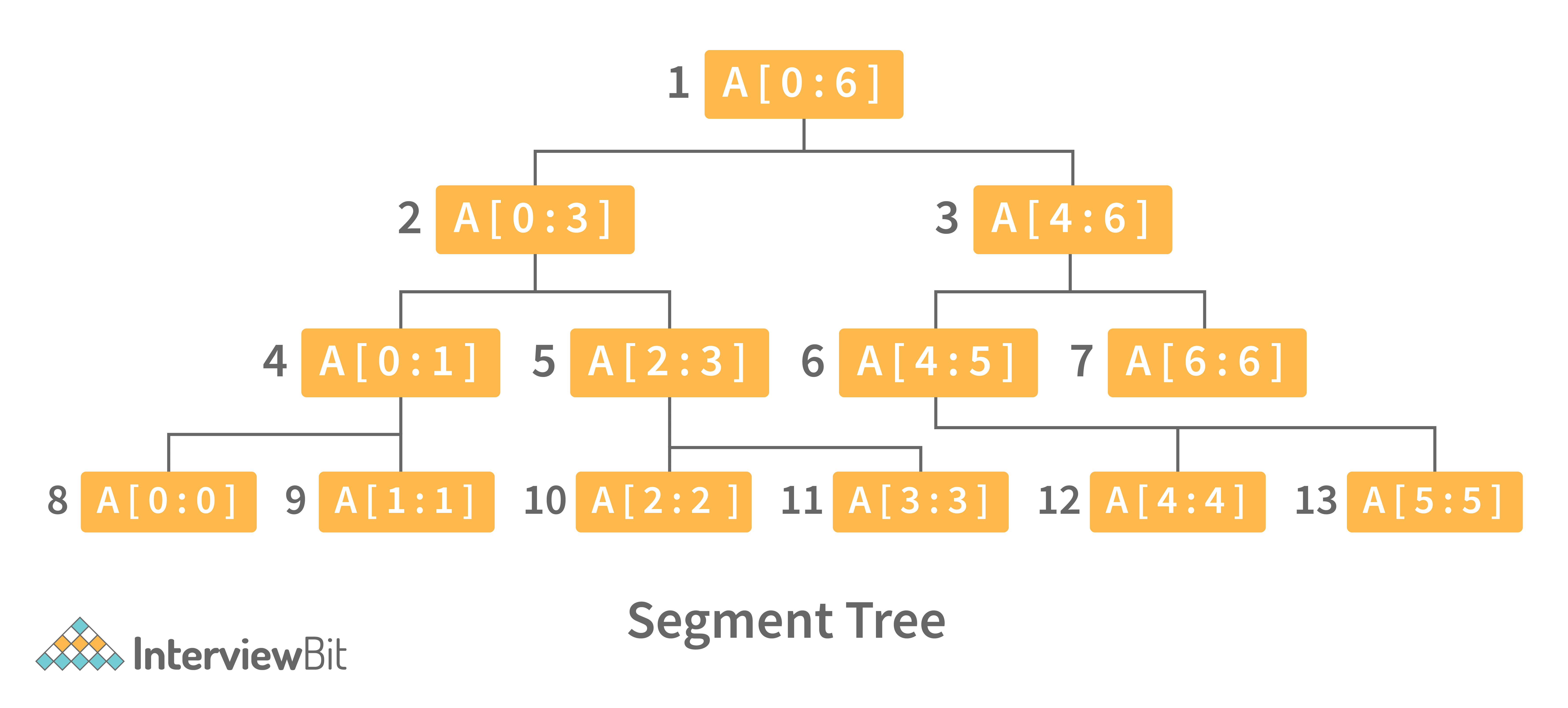
Following are key operations performed on the Segment tree data structure:
- Building Tree: In this step, we create the structure and initialize the segment tree variable.
- Updating the Tree: In this step, we change the tree by updating the array value at a point or over an interval.
- Querying Tree: This operation can be used to run a range query on the array.
Following are real-time applications for Segment Tree:
- Used to efficiently list all pairs of intersecting rectangles from a list of rectangles in the plane.
- The segment tree has become popular for use in pattern recognition and image processing.
- Finding range sum/product, range max/min, prefix sum/product, etc
- Computational geometry
- Geographic information systems
- Static and Dynamic RMQ (Range Minimum Query)
- Storing segments in an arbitrary manner
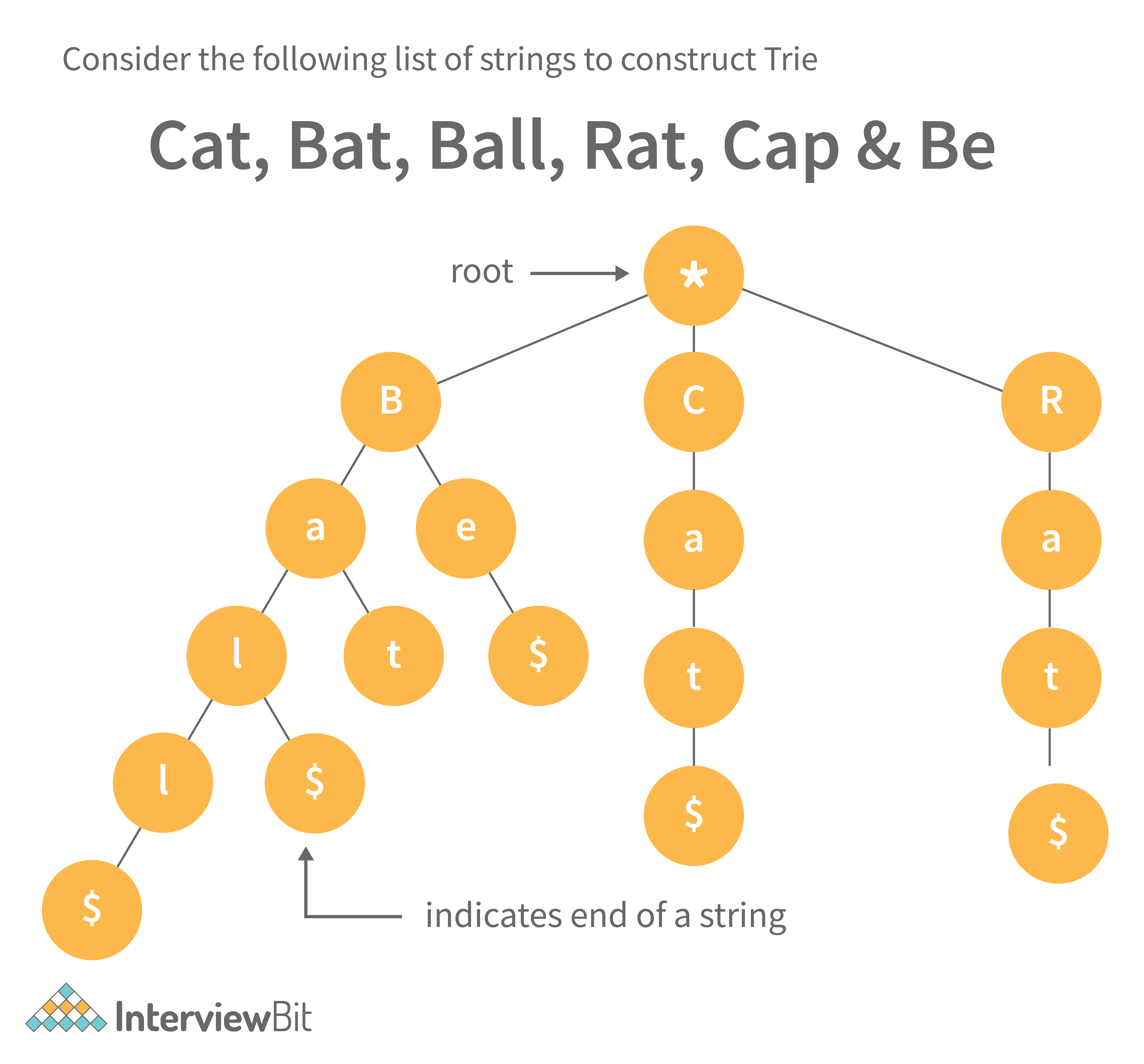
13. Define Trie data structure and its applications
The word "Trie" is an abbreviation for "retrieval." Trie is a data structure that stores a set of strings as a sorted tree. Each node has the same number of pointers as the number of alphabet characters. It can look up a word in the dictionary by using its prefix. Assuming that all strings are formed from the letters 'a' to 'z' in the English alphabet, each trie node can have a maximum of 26 points.
Trie is also referred to as the digital tree or the prefix tree. The key to which a node is connected is determined by its position in the Trie. Trie allows us to insert and find strings in O(L) time, where L is the length of a single word. This is clearly faster than BST. Because of how it is implemented, this is also faster than Hashing. There is no need to compute a hash function. There is no need to handle collisions (like we do in open addressing and separate chaining)
Another benefit of Trie is that we can easily print all words in alphabetical order, which is not easy with hashing. Trie can also perform prefix search (or auto-complete) efficiently.
The main disadvantage of tries is that they require a large amount of memory to store the strings. We have an excessive number of node pointers for each node
Following are some real-time applications for Trie data structure:
- Auto-Complete and Search for Search Engines
- Genome Analysis
- Data Analytics
- Browser History
- Spell Checker
14. Define Red-Black Tree and its applications
Red Black Trees are a type of self-balancing binary search tree. Rudolf Bayer invented it in 1972 and dubbed it "symmetric binary B-trees."
A red-black tree is a Binary tree in which each node has a colour attribute, either red or black. By comparing the node colours on any simple path from the root to a leaf, red-black trees ensure that no path is more than twice as long as any other, ensuring that the tree is generally balanced.
Red-black trees are similar to binary trees in that they both store their data in two's complementary binary formats. However, red-black trees have one important advantage over binary trees: they are faster to access. Because red-black trees are so fast to access, they are often used to store large amounts of data.
Red-black trees can be used to store any type of data that can be represented as a set of values.
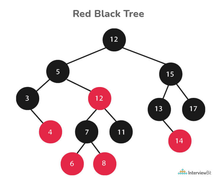
Every Red-Black Tree Obeys the Following Rules:
- Every node is either red or black.
- The tree's root is always black.
- There are no two red nodes that are adjacent.
- There is the same number of black nodes on every path from a node to any of its descendant's NULL nodes.
- All of the leaf nodes are black.
Following are some real-time applications for the Red-Black Tree data structure:
- The majority of self-balancing BST library functions in C++ or Java use Red-Black Trees.
- It is used to implement Linux CPU Scheduling.
- It is also used to reduce time complexity in the K-mean clustering algorithm in machine learning.
- MySQL also employs the Red-Black tree for table indexes in order to reduce searching and insertion time.
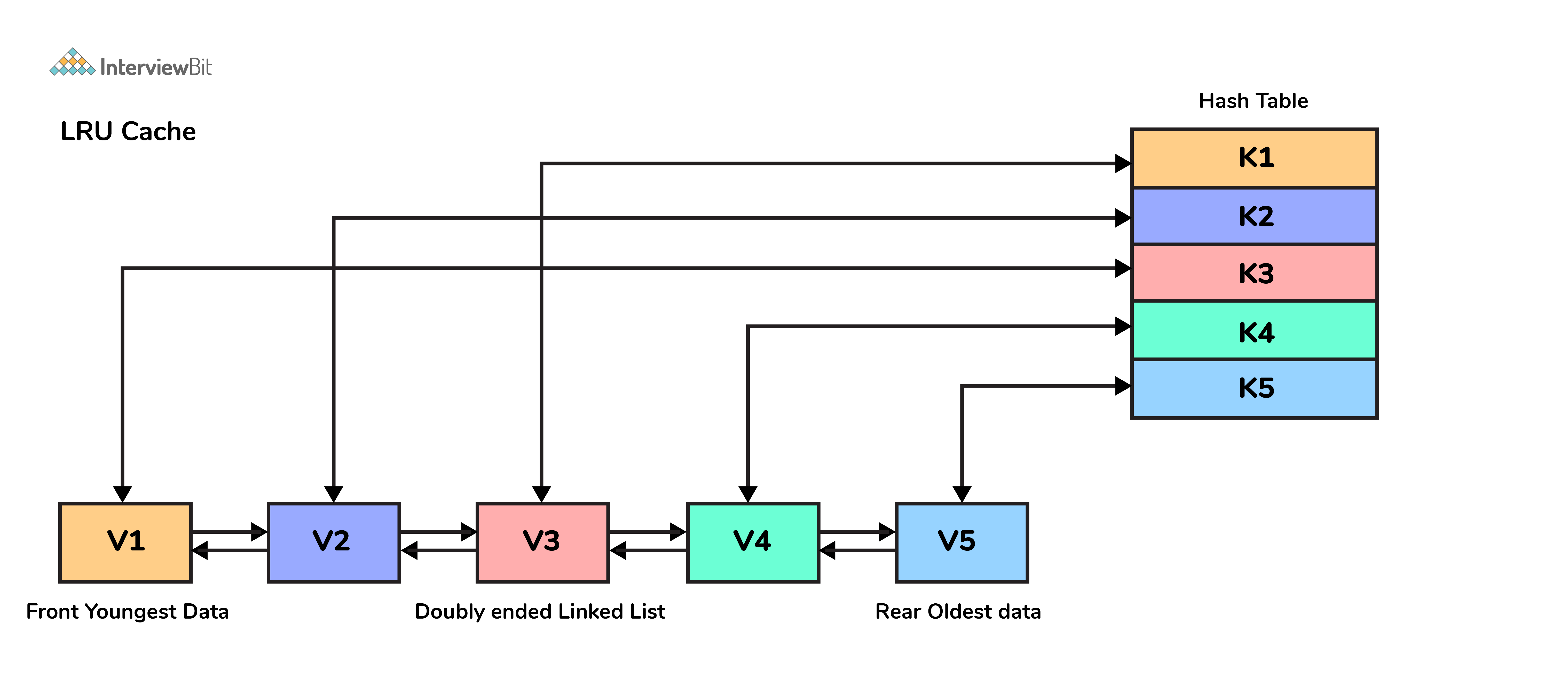
15. Which data structures are used for implementing LRU cache?
LRU cache or Least Recently Used cache allows quick identification of an element that hasn’t been put to use for the longest time by organizing items in order of use. In order to achieve this, two data structures are used:
- Queue – This is implemented using a doubly-linked list. The maximum size of the queue is determined by the cache size, i.e by the total number of available frames. The least recently used pages will be near the front end of the queue whereas the most recently used pages will be towards the rear end of the queue.
- Hashmap – Hashmap stores the page number as the key along with the address of the corresponding queue node as the value.
16. What is a heap data structure?
Heap is a special tree-based non-linear data structure in which the tree is a complete binary tree. A binary tree is said to be complete if all levels are completely filled except possibly the last level and the last level has all elements as left as possible. Heaps are of two types:
-
Max-Heap:
- In a Max-Heap the data element present at the root node must be the greatest among all the data elements present in the tree.
- This property should be recursively true for all sub-trees of that binary tree.
-
Min-Heap:
- In a Min-Heap the data element present at the root node must be the smallest (or minimum) among all the data elements present in the tree.
- This property should be recursively true for all sub-trees of that binary tree.
Data Structure Coding Interview Questions
1. Write a program to remove duplicates from a sorted array in place?
- Input: {1, 1, 1, 2, 3, 3, 6, 6, 7}
- Output: {1, 2, 3, 6, 7}
- Explanation: The given input has only 1,2,3,6, and 7 as unique elements, hence the output only lists them out.
#include <bits/stdc++.h>
using namespace std;

class Solution{
public:
    //function that takes an array and its size as arguments
    int removeDuplicates(int a[],int n){
        int index=0;
        for(int i=1;i<n;i++) {

            if(a[i]!=a[index]) { //change index
                index++; //swap next line
                a[index]=a[i];
            }
          }
          return index+1;
    }
};

int main()
{
    int T;
    //taking the number of test cases from user
    cin>>T;
    //running the loop for all test cases
    while(T--)
    {
        int N;
        //taking size input from user
        cin>>N;
        int a[N];
        //taking array input from user
        for(int i=0;i<N;i++)
        {
            cin>>a[i];
        }
        Solution ob;
        //calling the removeDuplicates in the Solution class
        int n = ob.removeDuplicates(a,N);
        //printing the array after removing duplicates
        for(int i=0;i<n;i++)
            cout<<a[i]<<" ";
            cout<<endl;
        }
}- Time Complexity: O(n)
- Space Complexity: O(1)
2. Write a function for zigzag traversal in a binary tree
- Input:
- Output: [1, 3, 2, 4, 5, 6, 8, 7]
- Explanation: Zigzag Traversal first iterates the given level of the tree from left to right and then the next level as the right to the level.
// Tree Node
struct Node {
    int data;
    Node* left;
    Node* right;
};

//Function to store the zigzag order traversal of a tree in a list.
    vector <int> zigZagTraversal(Node* root)
    {
     //creating two stacks for level traversals in both order
    	stack<Node*> st1;
    	stack<Node*> st2;
     //vector to store the zigzag traversal
    	vector<int> result;

     //Initialize the first stack with the root element
    	st1.push(root);

     //Iterate until either of the stack is not empty
    	while(!st1.empty() || !st2.empty()){
        //iterate until the first stack is not empty
    	    while(!st1.empty()){
    	        Node* temp=st1.top();
    	        st1.pop();
    	        result.push_back(temp->data);

    	        if(temp->left)
    	            st2.push(temp->left);
    	        if(temp->right)
    	            st2.push(temp->right);
    	    }
         //Iterate until the second stack is not empty
    	    while(!st2.empty()){
    	        Node* temp=st2.top();
    	        st2.pop();
    	        result.push_back(temp->data);

    	        if(temp->right)
    	            st1.push(temp->right);
    	        if(temp->left)
    	            st1.push(temp->left);

    	    }
    	}
    	return result;
}- Time Complexity: O(n)
- Space Complexity: O(n)
3. Write a function to sort a linked list of 0s, 1s and 2s
- Input: 0->1->0->2->1->0->2->1
- Output: 0->0->0->1->1->1->2->2
- Explanation: All 0’s will come first then 1s and then 2s. This can be done in O(n) time by counting the occurrences of all three and rearranging them in the linked list.
//structure of the linked list
struct Node {
   int data;
   Node *left;
   Node *right;
}
//function take the head of the linked list as a parameter
void sortList(Node *head)
{
   //if linked list is empty then return back
   if(head==NULL)
       return;
   else
   {
       Node *temp=head;
       Node *temp1=head;
       //to store count of 0s, 1s, and 2s
       int count0=0,count1=0,count2=0;
       //calculating the count of 0s, 1s, and 2s
       while(temp!=NULL)
       {
           if(temp->data==0)
               count0++;
           else if(temp->data==1)
               count1++;
           else
               count2++;
           temp=temp->next;
       }
       //iterating over count of 0s and filling the linked list
       while(count0!=0)
       {
           temp1->data=0;
           temp1=temp1->next;
           count0--;
       }
     //iterating over count of 1s and filling the linked list
       while(count1!=0)
       {
           temp1->data=1;
           temp1=temp1->next;
           count1--;
       }
     //iterating over count of 2s and filling the linked list
       while(count2!=0)
       {
           temp1->data=2;
           temp1=temp1->next;
           count2--;
       }
   }
}- Time Complexity: O(n)
- Space Complexity: O(1)
4. Write a function to detect cycle in an undirected graph
- Input: n = 4, e = 4 , 0 1, 1 2, 2 3, 3 1
- Output: Yes
-
Explanation: The graph is represented as follows in adjacency list representation:
0->1
1->2
2->3
3->1
From the above representation, we can see that there exists a cycle: 1→2→3→1
//function to run dfs for a given node in the graph
  int dfs(int v,vector<int> adj[],vector<int> &visited,vector<int> &rec,int i,int parent){
        int ans=0;
        visited[i]=1;
        rec[i]=1;
        for(auto x : adj[i]){
            if(x!=parent) {
                if(rec[x])
                    return 1;
                ans=dfs(v,adj,visited,rec,x,i);
                if(ans)
                   return 1;
            }
        }
        rec[i]=0;
        return 0;
    }
    // Function to detect cycle in an undirected graph.
    // it takes adjacency list representation as an argument
    bool isCycle(int v, vector<int> adj[]) {
        vector<int> visited(v,0),rec(v,0);
        int ans=0;
        for(int i=0;i<v;i++){
            if(visited[i]==0)
                ans=dfs(v,adj,visited,rec,i,-1);
            if(ans)
                return 1;
        }
        return 0;
}- Time Complexity: O(V+E)
- Space Complexity: O(V)
5. Write a function to convert an infix expression to postfix expression
- Input: a+b*(c^d)
- Output: abcd^*+
int prec(char c)
{
    if (c == '^')
        return 3;
    else if (c == '/' || c == '*')
        return 2;
    else if (c == '+' || c == '-')
        return 1;
    else
        return -1;
}
  public:
    // Function to convert an infix expression to a postfix expression.
    string infixToPostfix(string s) {
        stack<char> st; // For stack operations, we are using C++ built in stack
        string result;

        for (int i = 0; i < s.length(); i++) {
            char c = s[i];

            // If the scanned character is
            // an operand, add it to the output string.
            if ((c >= 'a' && c <= 'z') || (c >= 'A' && c <= 'Z')
            || (c >= '0' && c <= '9'))
                result += c;

            // If the scanned character is an
            // '(', push it to the stack.
            else if (c == '(')
                st.push('(');

            // If the scanned character is an ')',
            // pop and to output string from the stack
            // until an '(' is encountered.
            else if (c == ')') {
                while (st.top() != '(') {
                    result += st.top();
                    st.pop();
                }
                st.pop();
            }

            // If an operator is scanned
            else {
                while (!st.empty()
                   && prec(s[i]) <= prec(st.top())) {
                    if (c == '^' && st.top() == '^')
                        break;
                    else {
                        result += st.top();
                        st.pop();
                    }
                }
                st.push(c);
            }
        }

        // Pop all the remaining elements from the stack
        while (!st.empty()) {
            result += st.top();
            st.pop();
        }

        return result;
}- Time Complexity: O(n)
- Space Complexity: O(n)
6. Write a function to find the maximum for each and every contiguous subarray of size k.
- Input: N = 9, K = 3 arr[] = {1, 2, 3, 1, 4, 5, 2, 3, 6}
- Output: {3, 3, 4, 5, 5, 5, 6}
- Explanation: In the first subarray of size 3: {1,2,3}, the value 3 is maximum, similarly for all such subarrays for size 3.
//function to find maximum in each subarray using sliding window approach
vector<int> max_of_subarrays(vector<int> arr, int n, int k){
        int i=0,j=0;
        deque<int> dq;
        dq.push_front(i++);
        while(i<k)
        {
            while(!dq.empty()&&arr[dq.back()]<=arr[i])
            dq.pop_back();
            dq.push_back(i++);
        }
        vector<int> ans;
        while(i<n)
        {
            ans.push_back(arr[dq.front()]);
            while(!dq.empty()&&j>=dq.front())
            {
                dq.pop_front();

            }
            j++;
             while(!dq.empty()&&arr[dq.back()]<=arr[i])
            dq.pop_back();
            dq.push_back(i++);
        }
        ans.push_back(arr[dq.front()]);
        return ans;

}- Time Complexity: O(n)
- Space Complexity: O(k)
7. Write a function to merge two sorted binary search tree
Input:
First BST
7
/ \
5 9
Second BST
4
/ \
3 12
Output: 3 4 5 6 7 9 12
//Function to return a list of integers denoting the node
//values of both the BST in a sorted order.
    void inorder(Node*root,vector<int>&v){
        if(root==NULL)
            return;
        inorder(root->left,v);
        v.push_back(root->data);
        inorder(root->right,v);
    }
    vector<int> merge(vector<int>v1,vector<int>v2){
        vector<int>v;
        int n1=v1.size(),n2=v2.size(),i=0,j=0;
        while(i<n1&&j<n2){
            if(v1[i]>v2[j]){
                v.push_back(v2[j]);
                j++;
            }
            else{
                v.push_back(v1[i]);
                i++;
            }
        }
        while(i<n1){
            v.push_back(v1[i]);
            i++;
        }
        while(j<n2){
            v.push_back(v2[j]);
            j++;
        }
        return v;
    }
    vector<int> merge(Node *root1, Node *root2)
    {
       vector<int>v1,v2;
       inorder(root1,v1);
       inorder(root2,v2);
       return merge(v1,v2);
}- Time Complexity: O(m+n)
- Space Complexity: O(height of the first tree + height of the second tree)
8. Write a function to print all unique rows of the given matrix.
Input:
{{1, 1, 1, 0, 0},
{0, 1, 0, 0, 1},
{1, 0, 1, 1, 0},
{0, 1, 0, 0, 1},
{1, 1, 1, 0, 0}}
Output:
{{1, 1, 1, 0, 0},
{0, 1, 0, 0, 1},
{1, 0, 1, 1, 0}}
vector<vector<int>> uniqueRow(int M[MAX][MAX],int row,int col)
{
set<vector<int>> st;
vector<vector<int>> v;

for(int i=0; i<row; i++) {
    vector<int> v1;
    for(int j=0; j<col; j++) {
        v1.push_back(M[i][j]);
    }
    if(st.count(v1) == 0) {
         v.push_back(v1);
         st.insert(v1);
    }
}

return v;
}- Time Complexity: O( ROW x COL )
- Space Complexity: O( ROW )
9. Write a function to find number of subarrays with product less than K
- Input: arr = [1, 6, 2, 3, 2, 1], k = 12
- Output: 11
int numSubarrayProductLessThanK(vector<int>& nums, int k) {
        int ans=0;
        int pdt=1;
        int left=0,right=0;
        while(right<=nums.size()-1){

            pdt*=nums[right];
            while(pdt>=k and left<nums.size()){
                pdt/=nums[left];
                left++;

            }
            if(right-left>=0)
            ans+=right-left+1;//since on adding a new element new subarrays formed is r-i+1;
            right++;

        }
        return ans;
}- Time Complexity: O(n)
- Space Complexity: O(1)
10. Find the subsequence of length 3 with the highest product from a sequence of non-negative integers, with the elements in increasing order.
- Input: n = 8 arr[ ] = {6, 7, 10, 1, 2, 3, 11, 12}
- Output: {10, 11, 12}
The three increasing elements of the given arrays are 10, 11, and 12, which form a three-size subsequence with the highest product.
 vector<int> maxProductSubsequence(int *a , int n)
    {
        set<int> s;
        long long largestOnLeft[n];
        for(int i=0;i<n;i++)
        {
            s.insert(a[i]);
            auto it=s.lower_bound(a[i]);
            if(it==s.begin())
            {
                largestOnLeft[i]=-1;
                continue;
            }
            it--;
            largestOnLeft[i]=*it;
        }
        int m=0;
        long long p=INT_MIN;
        vector<int> result(3);
        result[0]=-1;
        for(int i=n-1;i>=0;i--)
        {
          if(a[i]>=m){
          m=a[i];}
          else
          {
              if(largestOnLeft[i] !=-1)
              {
                  if(largestOnLeft[i]*a[i]*m >p)
                  {
                      p=largestOnLeft[i]*a[i]*m;
                      result[0]=largestOnLeft[i];
                      result[1]=a[i];
                      result[2]=m;
                  }
              }
          }
        }
        return v;
}- Time Complexity: O(nlog(n))
- Space Complexity: O(n)
11. Write a function to implement Quicksort on Doubly Linked List
- Input: 8<->10<->1<->7<->6
- Output: 1<->6<->7<->8<->10
class Solution{
public:
    Node* partition(Node *l, Node *h){
        //Your code goes here
        Node*temp = h;
        Node*tt = l;
        Node*first = l;

        while(tt != h){
              if(tt->data <= temp->data){
                  swap(first->data, tt->data);
                  first = first->next;
              }
              tt = tt -> next;
        }
        swap(first-> data, h->data);
        return first;

    }
};

void _quickSort(struct Node* l, struct Node *h)
{
    if (h != NULL && l != h && l != h->next)
    {
        Solution ob;
        struct Node *p = ob.partition(l, h);
        _quickSort(l, p->prev);
        _quickSort(p->next, h);
    }
}

void quickSort(struct Node *head)
{
    struct Node *h = lastNode(head);
    _quickSort(head, h);
}- Time Complexity: O(n^2) in the worst case when the list is already sorted. O(nlog(n)) in the best and average case.
- Space Complexity: O(n)
12. Write a function to connect nodes at the same level of a binary tree
Input: 100
/ \
13 15
/ \ \
14 1 20
Output: 100-> NULL
/ \
13 -> 15 -> NULL
/ \ \
14 -> 1 -> 20 -> NULL
class Solution
{
    public:
    //Function to connect nodes at the same level.
    void connect(Node *p)
    {
       map<int,vector<Node *> > m;
       queue<Node *> q;
       queue<int> l;
       q.push(p);
       l.push(0);
       while(!q.empty())
       {
           Node *temp=q.front();
           int level=l.front();
           q.pop();
           l.pop();
           m[level].push_back(temp);
           if(temp->left!=NULL)
           {
               q.push(temp->left);
               l.push(level+1);
           }
           if(temp->right!=NULL)
           {
               q.push(temp->right);
               l.push(level+1);
           }
       }
       for(map<int,vector<Node *> > ::iterator it=m.begin();it!=m.end();it++)
       {
           vector<Node *> temp1=it->second;
           for(int i=0;i<temp1.size()-1;i++)
           {
               temp1[i]->nextRight=temp1[i+1];
           }
           temp1[temp1.size()-1]->nextRight=NULL;
       }
    }
};- Time Complexity: O(n)
- Space Complexity: O(n)
13. Write a function to find number of structurally unique binary trees are possible
Input: N = 3
Output: 5 for N = 3, there are 5 possible BSTs:
1 3 3 2 1
\ / / / \ \
3 2 1 1 3 2
/ / \ \
2 1 2 3
class Solution
{
    public:
     //function to calculate binomial coefficient C(n,k)
    long long int binomialCoefficient(long long int n, long long int k)
    {
        long long int res = 1;
        if (k > n - k)
            k = n - k;

        for (long long int i = 0; i < k; ++i)
        {
            res *= (n - i);
            res /= (i + 1);
        }

        return res;
    }

   //function to calculate Nth Catalan Number
    long long int catalanNumber(long long in n)
    {
        // Calculate value of 2nCn
        long long int C = binomialCoefficient(2*n, n);

        // return 2nCn/(n+1)
        return C/(n+1);
    }

    //Function to return the total number of possible unique BST.
    long long int numOfUniqueBinarySearchTrees(int n)
    {
         // find nth catalan number
        long long int countOfUniqueBinarySearchTrees = catalanNumber(n);

        // return nth catalan number
        return countOfUniqueBinarySearchTrees;
    }
};- Time Complexity: O(n)
- Space Complexity: O(1)
14. Implement LRU(Least Recently Used) Cache
class LRUCache
{
    private:
    class node_t {
        public:
        int key;
        int value;
        node_t * next;
        node_t * prev;
    };

    int cap;
    node_t head;
    unordered_map<int, node_t*> tbl;

    void remove_node(node_t * node) {
        node->next->prev = node->prev;
        node->prev->next = node->next;
    }
    void add_node(node_t * node) {
        node->next = head.next;
        node->prev = &head;
        head.next = node;
        node->next->prev = node;
    }
    public:
    //Constructor for initializing the cache capacity with the given value.
    LRUCache(int cap): cap(cap)
    {
        // code here
        head.prev = &head;
        head.next = &head;
    }

    //Function to return value corresponding to the key.
    int get(int key)
    {
        // your code here
        unordered_map<int, node_t*>::iterator it = tbl.find(key);
        if(it==tbl.end())
            return -1;
        remove_node(it->second);
        add_node(it->second);
        return it->second->value;
    }

    //Function for storing key-value pair.
    void set(int key, int value)
    {
        // your code here
        unordered_map<int, node_t*>::iterator it = tbl.find(key);
        if(it!=tbl.end())
        {
            remove_node(it->second);
            add_node(it->second);
            it->second->value = value;
        }
        else {
            node_t * node = new node_t;
            node->key = key;
            node->value = value;
            add_node(node);
            tbl[key] = node;
            if(tbl.size()>cap) {
                auto * old_node = head.prev;
                tbl.erase(old_node->key);
                remove_node(old_node);
                delete old_node;
            }
        }
    }
};- Time Complexity: O(1) to get an element
- Space Complexity: O(n)
15. Write a function to determine whether duplicate elements in a given array are within a given distance of each other.
- Input: arr[] = {1, 2, 3, 4, 2, 1, 2} range=3
- Output: True
class Solution {
    public:

    bool checkDuplicatesWithinRange(vector<int> arr, int range)
    {
        // Creating an empty hashset
        unordered_set<int> myset;

        // Traversing the input array
        for (int i = 0; i < arr.size(); i++)
        {
            // If already present in hashset, then we found a duplicate within range distance
            if (myset.find(arr[i]) != myset.end())
                return true;

            // Add this item to hashset
            myset.insert(arr[i]);

            // Remove the range+1 distant item from the hashset
            if (i >= range)
                myset.erase(arr[i-range]);
        }
        return false;
    }
};- Time Complexity: O(n)
- Space Complexity: O(n)
16. Write a recursive function to calculate the height of a binary tree in Java.
- Consider that every node of a tree represents a class called Node as given below:
public class Node{
     int data;
     Node left;
     Node right;
}- Then the height of the binary tree can be found as follows:
     int heightOfBinaryTree(Node node)
     {
         if (node == null)
             return 0; // If node is null then height is 0 for that node.
         else
         {
             // compute the height of each subtree
             int leftHeight = heightOfBinaryTree(node.left);
             int rightHeight = heightOfBinaryTree(node.right);
             //use the larger among the left and right height and plus 1 (for the root)
             return Math.max(leftHeight, rightHeight) + 1;
         }
     }
17. Write Java code to count number of nodes in a binary tree
int countNodes(Node root)
{
    int count =  1;             //Root itself should be counted
    if (root ==null)
        return 0;
    else
    {
        count += countNodes(root.left);
        count += countNodes(root.right);
        return count;
    }
}
18. Print Left view of any binary trees.
- The main idea to solve this problem is to traverse the tree in pre order manner and pass the level information along with it. If the level is visited for the first time, then we store the information of the current node and the current level in the hashmap. Basically, we are getting the left view by noting the first node of every level.
- At the end of traversal, we can get the solution by just traversing the map.
- Consider the following tree as example for finding the left view:
- Left view of a binary tree in Java:
 import java.util.HashMap;

  //to store a Binary Tree node
  class Node
  {
      int data;
      Node left = null, right = null;

      Node(int data) {
          this.data = data;
      }
  }
  public class InterviewBit
  {
      // traverse nodes in pre-order way
      public static void leftViewUtil(Node root, int level, HashMap<Integer, Integer> map)
      {
          if (root == null) {
              return;
          }

          // if you are visiting the level for the first time
          // insert the current node and level info to the map
          if (!map.containsKey(level)) {
              map.put(level, root.data);
          }

          leftViewUtil(root.left, level + 1, map);
          leftViewUtil(root.right, level + 1, map);
      }

      // to print left view of binary tree
      public static void leftView(Node root)
      {
          // create an empty HashMap to store first node of each level
          HashMap<Integer, Integer> map = new HashMap<>();

          // traverse the tree and find out the first nodes of each level
          leftViewUtil(root, 1, map);

          // iterate through the HashMap and print the left view
          for (int i = 0; i <map.size(); i++) {
              System.out.print(map.get(i) + " ");
          }
      }

      public static void main(String[] args)
      {
          Node root = new Node(4);
          root.left = new Node(2);
          root.right = new Node(6);
          root.left.left = new Node(1);
          root.left.left = new Node(3);
          root.right.left = new Node(5);
          root.right.right = new Node(7);
          root.right.left.left = new Node(9);

          leftView(root);
      }
  }
19. Given an m x n 2D grid map of '1’s which represents land and '0’s that represents water return the number of islands (surrounded by water and formed by connecting adjacent lands in 2 directions - vertically or horizontally).
Assume that the boundary cases - which are all four edges of the grid are surrounded by water.
Constraints are:
m == grid.length
n == grid[i].length
1 <= m, n <= 300
grid[i][j] can only be ‘0’ or ‘1’.
Example:
Input: grid = [
[“1” , “1” , “1” , “0” , “0”],
[“1” , “1” , “0” , “0” , “0”],
[“0” , “0” , “1” , “0” , “1”],
[“0” , “0” , “0” , “1” , “1”]
]
Output: 3
class InterviewBit {
    public int numberOfIslands(char[][] grid) {
        if(grid==null || grid.length==0||grid[0].length==0)
            return 0;

        int m = grid.length;
        int n = grid[0].length;

        int count=0;
        for(int i=0; i<m; i++){
            for(int j=0; j<n; j++){
                if(grid[i][j]=='1'){
                    count++;
                    mergeIslands(grid, i, j);
                }
            }
        }

        return count;
    }

    public void mergeIslands(char[][] grid, int i, int j){
        int m=grid.length;
        int n=grid[0].length;

        if(i<0||i>=m||j<0||j>=n||grid[i][j]!='1')
            return;

        grid[i][j]='X';

        mergeIslands(grid, i-1, j);
        mergeIslands(grid, i+1, j);
        mergeIslands(grid, i, j-1);
        mergeIslands(grid, i, j+1);
    }
}
20. What is topological sorting in a graph?
- Topological sorting is a linear ordering of vertices such that for every directed edge ij, vertex i comes before j in the ordering.
- Topological sorting is only possible for Directed Acyclic Graph (DAG).
- Applications:
- jobs scheduling from the given dependencies among jobs.
- ordering of formula cell evaluation in spreadsheets
- ordering of compilation tasks to be performed in make files,
- data serialization
- resolving symbol dependencies in linkers.
- Topological Sort Code in Java:
// V - total vertices
     // visited - boolean array to keep track of visited nodes
     // graph - adjacency list.
    // Main Topological Sort Function.
    void topologicalSort()
    {
        Stack<Integer> stack = new Stack<Integer>();

        // Mark all the vertices as not visited
        boolean visited[] = new boolean[V];
        for (int j = 0; j < V; j++){
            visited[j] = false;
        }
        // Call the util function starting from all vertices one by one
        for (int i = 0; i < V; i++)
            if (visited[i] == false)
                topologicalSortUtil(i, visited, stack);

        // Print contents of stack -> result of topological sort
        while (stack.empty() == false)
            System.out.print(stack.pop() + " ");
    }

    // A helper function used by topologicalSort
    void topologicalSortUtil(int v, boolean visited[],
                             Stack<Integer> stack)
    {
        // Mark the current node as visited.
        visited[v] = true;
        Integer i;

        // Recur for all the vertices adjacent to the current vertex
        Iterator<Integer> it = graph.get(v).iterator();
        while (it.hasNext()) {
            i = it.next();
            if (!visited[i])
                topologicalSortUtil(i, visited, stack);
        }

        // Push current vertex to stack that saves result
        stack.push(new Integer(v));
    }
Conclusion
In this post, we covered the most important and frequently asked Data Structures interview questions. We've also included some pointers and tricks to help you prepare for the interview. When preparing for the product-based companies interview, keep in mind that the Data Structures interview is a critical component of the process. It is critical that you are well prepared for the interview because it will determine whether or not you are hired. As a result, it is critical to begin planning as soon as possible.
Additional Interview Resources
- Programming: DSA - https://www.interviewbit.com/courses/programming/
- Data Structure MCQ - https://www.interviewbit.com/data-structure-mcq/
- Best Books for Data Structures and Algorithms - https://www.interviewbit.com/blog/data-structures-and-algorithms-books/
- Best Data Structures and Algorithms Course - https://www.interviewbit.com/blog/best-courses-for-data-structures-and-algorithms/
- Free Java DSA Certification Course - https://www.scaler.com/topics/course/dsa-beginners-java/
- Algorithm Interview Questions - https://www.interviewbit.com/algorithm-interview-questions/
- Master Data Structures and Algorithms With the Scaler Academy Program - https://www.scaler.com/courses/data-structures-and-algorithms/
- Difference Between Array and Linked List - https://www.scaler.com/topics/difference-between-array-and-linked-list/
InterviewBit Data Structure Interview Questions
1. Explain time complexity and Big O notation with examples.
Time complexity shows how the number of operations in an algorithm increases as the input size increases. It helps us understand how the algorithm will perform for large inputs.
Big O notation is used to represent this growth. It shows the upper bound (worst-case) of an algorithm. It does not measure actual time. Instead, it focuses on how the number of steps grows with n.
Did you know? That Big O notation is part of asymptotic analysis, which studies the behaviour of algorithms as input size approaches infinity.
While writing Big O:
- Constants are ignored
- Lower-order terms are ignored
- Only the dominant term is considered
This is done because, for large inputs, smaller terms do not significantly affect performance.
These are some of the common time complexities that you should keep in mind -
- O(1) - constant time (e.g., accessing an element in a hash table)
- O(n log n) - linearithmic time (e.g., merge sort)
- O(log n) - logarithmic time (e.g., binary search)
- O(n) - linear time (e.g., traversing an array)
- O(n²) - nested loops
- O(n3) - Cubic time
- O(2ⁿ) - exponential (e.g., recursive Fibonacci)
- O(n!) - Factorial time
Here’s an example:
def count_pairs(arr):

    n = len(arr)

    for i in range(n):

        for j in range(n):

            print(arr[i], arr[j])
The outer loop runs n times.
The inner loop also runs n times for each iteration.
Total operations = n × n
This results in quadratic growth, so the time taken increases proportionally to n².
Space complexity is analyzed similarly. It represents how much additional memory is required. For example, if an algorithm uses an extra array of size n, the space complexity is O(n). Recursive algorithms also use space due to the call stack.
Some algorithms have different complexities based on input. For example, quicksort runs in O(n log n) on average but can degrade to O(n²) in the worst case.
2. Compare common sorting algorithms: when to use which?
Sorting algorithms are used to arrange elements in a specific order, i.e, usually ascending or descending. Different algorithms are used based on time complexity, space usage, and stability.
You can look into this table below for a detailed comparison -
| Algorithm | Running Time | What they do |
|---|---|---|
| Bubble Sort | O(n²) | This algorithm repeatedly compares adjacent elements and swaps them if they are in the wrong order. It is simple to understand, but it becomes very slow as the input size increases. It may still work for very small datasets or when the data is almost sorted. |
| Merge Sort | O(n log n) | Merge sort divides the array into smaller parts, sorts them separately, and then merges them back together. It always runs in O(n log n) time and maintains the relative order of equal elements for stability. But do keep in mind that it needs extra memory. |
| Quick Sort | O(n log n) average, O(n²) worst | Quick sort selects a pivot and partitions the array around it. In most cases, it performs very fast, and because of that, it is very commonly used while working. But one thing you need to ensure is that if the pivot is not chosen properly, the performance can degrade to O(n²). |
| Heap Sort | O(n log n) | Heap sort uses a binary heap to repeatedly extract the maximum or minimum element. It guarantees O(n log n) time in all cases and does not require extra space, but it is not stable and is usually less preferred than quicksort in practice. |
| Counting Sort | O(n + k) | Counting sort does not compare elements. Instead, it counts the frequency of each value and uses this information to place elements in order. It works well when the range of input values is small, but it is not suitable for large ranges. |
| Radix Sort | O(nk) | Radix sort processes numbers digit by digit, usually starting from the least significant digit. It is efficient for integers or fixed-length data. Its performance depends on the number of digits, and it is often combined with counting sort internally. |
Please note -
- Stable sorting means equal elements keep their original order
- In-place sorting means no extra memory is required
- Comparison-based sorts cannot be faster than O(n log n) in general
Here’s an example you can refer to - Quick sort works using the divide-and-conquer approach.
It selects a pivot and partitions the array into two parts:
- Elements smaller than pivot
- Elements greater than pivot
def quicksort(arr, low, high):

    if low < high:

        pivot_index = partition(arr, low, high)

        quicksort(arr, low, pivot_index - 1)

        quicksort(arr, pivot_index + 1, high)

def partition(arr, low, high):

    pivot = arr[high]

    i = low - 1


    for j in range(low, high):

        if arr[j] < pivot:

            i += 1

            arr[i], arr[j] = arr[j], arr[i]


    arr[i + 1], arr[high] = arr[high], arr[i + 1]

    return i + 1
Time Complexity:
- Average case - O(n log n)
- Worst case - O(n²) (when pivot is poorly chosen)
Space Complexity: O(log n) (due to recursion)
When to Use Which Algorithm
- Use merge sort when you require stability
- Use quicksort for fast performance in most cases
- Use heap sort when worst-case O(n log n) is required
- Use counting/radix sort when data is within a fixed range
- Avoid bubble sort for large inputs
Also remember -
When you use applications, built-in sorting functions (like Python’s sort()) use optimized algorithms such as Timsort, which combines merge sort and insertion sort.
3. Explain binary search. When can you apply it beyond sorted arrays?
Binary search uses the concept of divide and conquer and works by repeatedly dividing the search space in half to find an element. It works on a sorted dataset. It works by comparing the target with the middle element and deciding which half to continue searching in, so that there is no need to search each and every element.
Here’s how Binary search works -
- Start with two pointers: left = 0 and right = n - 1
- Will find the middle element
- If the target matches - return index
- If the target is smaller, search in the left half
- If the target is larger, search in the right half
This will repeat until the element is found or the range becomes invalid
Here’s an example code for your reference -
def binary_search(arr, target):

    left = 0

    right = len(arr) - 1


    while left <= right:

        mid = left + (right - left) // 2


        if arr[mid] == target:

            return mid

        elif arr[mid] < target:

            left = mid + 1

        else:

            right = mid - 1


return -1- Time complexity - O(log n)
- Space complexity - O(1)
Important detail - Please keep this in mind: Binary search works only when the data is sorted or arranged in a way where one half can be eliminated at each step.
Also, to avoid overflow in some languages, mid is calculated as: mid = left + (right - left) // 2
Binary search can be utilized for various other aspects involving a monotonic pattern, which means that as the input increases, the output either only increases or only decreases.
Here are some common mistakes that you should avoid making -
- Using binary search on unsorted data
- Incorrect loop condition (< vs <=)
- Wrong pointer updates leading to an infinite loop
- Off-by-one errors
Always remember that binary search is best to use whenever you can reduce the search space by half at every step, and not just anytime when working with sorted arrays.
4. What is dynamic programming? Explain with a classic example.
Dynamic programming is a technique used to solve problems by breaking them into smaller subproblems and storing their results. This avoids repeating the same computation again and again.
It is mainly used when the problem has overlapping subproblems and the problem has optimal substructure.
So, here’s what you should understand -
You need to store the result and reuse it so that you can avoid solving the subproblems multiple times.
There are two approaches:
- Top-down (memoization): recursion + storing results
- Bottom-up (tabulation): iterative solution using a table
Now, I’ll be giving some examples so that you have a better understanding. Here you go -
One of the most classic examples is Fibonacci
1. Simple Recursion (Inefficient)
def fib(n):

    if n <= 1:

        return n

    return fib(n-1) + fib(n-2)
Here, the same values are calculated multiple times.
For example, fib(3) is computed again and again.
Time Complexity: O(2ⁿ)
Space Complexity: O(n) (due to recursion stack)
2. Using Dynamic Programming (Optimized)
def fib(n):

    if n <= 1:

        return n


    dp = [0] * (n + 1)

    dp[0], dp[1] = 0, 1


    for i in range(2, n + 1):

        dp[i] = dp[i-1] + dp[i-2]


    return dp[n]
Here, each value is computed only once and stored.
Time Complexity: O(n)
Space Complexity: O(n)
Space Optimization - In this case:
We only need the last two values:
def fib(n):

    if n <= 1:

        return n


    prev2, prev1 = 0, 1


    for i in range(2, n + 1):

        curr = prev1 + prev2

        prev2 = prev1

        prev1 = curr


    return prev1
Space Complexity: O(1)
Here are some areas where Dynamic Programming is used -
- Coin change problem
- 0/1 knapsack
- Climbing stairs
- Longest common subsequence
Remember that dynamic programming improves performance by storing intermediate results and avoiding repeated calculations.
5. What are greedy algorithms? When do they work and when do they fail?
A greedy algorithm makes the best possible choice at each step. It does not look at the full problem. It simply picks what seems optimal at the current moment. Hence, these local choices will lead to a globally optimal solution.
Greedy algorithm works when the problem satisfies -
- Greedy choice property - which means choosing the best option at each step, leading to the correct result
- Optimum substructure - this means, overall solution can be built from smaller optimal choices
We can take activity selection as an example here,
We are given activities with start and end times. The goal is to select the maximum number of non-overlapping activities.
Greedy approach:
- Sort activities by end time
- Always pick the activity that finishes earliest
def activity_selection(activities):

    activities.sort(key=lambda x: x[1])


    count = 1

    last_end = activities[0][1]


    for i in range(1, len(activities)):

        if activities[i][0] >= last_end:

            count += 1

            last_end = activities[i][1]


    return count
Time Complexity: O(n log n) (due to sorting)
Space Complexity: O(1)
You should also understand that greedy might fail at times. The reason is that the local choices do not lead to a global optimum.
If we take the 0/1 knapsack as an example - In this problem, we try to maximize value within a weight limit. Here, the Greedy approach would be to pick the highest value, and that in turn may not give the correct result. Because selecting one item may block a better combination later, and that is this problem can be solved using dynamic problem and not greedy.
So, if you get confused as to which to use where between greedy and dynamic problem solving, then just remember this -
- Greedy makes one choice at a time, faster and simpler
- DP explores all possibilities, gives the correct result, but takes more time
6. Explain recursion and backtracking with examples.
Recursion is a technique where a function calls itself to solve a smaller part of the same problem. It continues until a base condition is reached.
Backtracking is built on recursion. It tries a solution, and if it does not work, it goes back and tries a different option.
It is important to understand both with examples, so here you go -
1. Recursion
A recursive function has two main parts:
- Base case - stops the recursion
- Recursive case - reduces the problem size
If we take Factorial as an example,
def factorial(n):

    if n == 0:

        return 1

    return n * factorial(n - 1)
Here you can see that the function keeps calling itself with a smaller value until it reaches 0.
Time Complexity: O(n)
Space Complexity: O(n) (due to call stack)
2. Backtracking
Backtracking is used when we need to explore all possible solutions.
At each step, what happens is:
- Choose an option
- Explore further
- If it does not work, undo the choice and try another
For example, if we take Generating All Subsets
def subsets(nums):

    result = []


    def backtrack(start, path):

        result.append(path[:])


        for i in range(start, len(nums)):

            path.append(nums[i])

            backtrack(i + 1, path)

            path.pop()


    backtrack(0, [])

    return result
We can see here that we add an element, then explore further, and then remove it (backtrack)
Time Complexity: O(2ⁿ)
Space Complexity: O(n)
They work differently, of course, but explaining the difference becomes a little hard, right? So here’s what you can say when asked -
- Recursion solves a problem by reducing it, and is used in areas like tree traversal, factorial, and Fibonacci.
- Backtracking explores all possible choices and undoes decisions, and it is used in areas like N-Queens, permutations, subsets, sudoku.
Also, just keep in mind that Backtracking can be a little expensive since it is used to explore many possibilities. It is often used when we need all valid solutions instead of something singular.
7. What is the two-pointer technique? When do you use it?
The two-pointer technique is used to solve problems by maintaining two indices instead of one. These pointers move through the data in a controlled way to reduce unnecessary comparisons.
It is mainly used to improve time complexity from O(n²) to O(n) in many problems.
You can notice some common patterns here, such as -
1. Opposite directions: One pointer starts from the beginning, the other from the end. Pointers move based on a condition. It is used in Two Sum in a sorted array and for checking palindromes.
2. Same Direction: Both pointers start from the same side. Here, one moves faster than the other. And it is used in removing duplicates and detecting cycles in linked lists.
3. Sliding Window: One pointer expands the window. The other shrinks it when needed. It is used in subarray or substring problems.
Here’s an example: Two Sum in Sorted Array
def two_sum(arr, target):

    left = 0

    right = len(arr) - 1


    while left < right:

        current = arr[left] + arr[right]


        if current == target:

            return [left, right]

        elif current < target:

            left += 1

        else:

            right -= 1


    return [-1, -1]
Here, we avoid checking all pairs.
Instead, we move pointers based on whether the sum is too small or too large. This reduces the number of comparisons significantly.
So, these are the instances under which the two-pointer technique can work best -
- When the array is sorted or can be sorted
- When you need to find pairs or subarrays
- When reducing time complexity is important
- When the problem involves continuous elements
Hence, the two-pointer technique works by using the structure of the data to eliminate unnecessary checks, instead of trying all possible combinations.
8. What is the sliding window technique?
The sliding window technique is used to work with a range of elements (subarray or substring) instead of individual elements. Instead of recalculating results for every window, we move the window step by step and update the result efficiently.
It helps reduce unnecessary computations, especially in problems involving contiguous elements.
Here are the types of sliding window techniques -
1. Fixed-size window:
Here, the window size remains constant.
Example: Maximum sum of subarray of size k
In this case, when the window moves forward:
- Add the next element
- Remove the previous element
2. Variable-size window:
The window size changes based on a condition.
Example: Longest substring without repeating characters
Here,
- Expand the window until the condition breaks
- Then shrink it from the left
You can refer to this general template to understand it better -
def sliding_window(arr):

    left = 0


    for right in range(len(arr)):

        # include current element


        while condition_not_valid:

            # remove elements from left

            left += 1


        # update result
With this format, it will be rest assured that each element is processed only once while expanding and shrinking the window.
You can look into this example of Longest Substring Without Repeating Characters
def longest_unique_substring(s):

    char_set = set()

    left = 0

    max_length = 0


    for right in range(len(s)):

        while s[right] in char_set:

            char_set.remove(s[left])

            left += 1


        char_set.add(s[right])

        max_length = max(max_length, right - left + 1)


    return max_length
Now, what happens here is that the window expands when characters are unique, and it shrinks when a duplicate is found
Each character is added and removed at most once, so the overall processing remains linear.
9. Explain Dijkstra's algorithm for the shortest path.
Dijkstra’s algorithm is used to find the shortest distance from a source node to all other nodes in a weighted graph. It works only when all edge weights are non-negative.
It works by always picking the node with the smallest known distance and updating its neighbors.
Here’s how the algorithm works:
- Assign distance 0 to the source node
- Assign infinity to all other nodes
- Use a priority queue (min-heap) to store nodes based on distance
Then repeat:
- Pick the node with the smallest distance
- For each of its neighbors:
- Calculate new distance = current distance + edge weight
- If this distance is smaller, update it
- Mark the node as visited
This process continues until all nodes are processed.
Here is an example -
import heapq

def dijkstra(graph, start):

    distances = {node: float('inf') for node in graph}

    distances[start] = 0


    pq = [(0, start)]


    while pq:

        current_dist, node = heapq.heappop(pq)


        if current_dist > distances[node]:

            continue


        for neighbor, weight in graph[node]:

            distance = current_dist + weight


            if distance < distances[neighbor]:

                distances[neighbor] = distance

                heapq.heappush(pq, (distance, neighbor))


    return distances
In this approach, the priority queue ensures that we always process the closest node first. Each edge is relaxed only when a shorter path is found.
You need to remember that it works only for non-negative weights, uses a greedy approach, and that a priority queue improves efficiency.
When we look into time and space - Using a priority queue, time depends on processing all edges and nodes with heap operations, and extra space is used to store distance,s, and the queue
Also note -
If the graph has negative edge weights, Dijkstra’s algorithm does not give correct results. In such cases, algorithms like Bellman-Ford are used.
10. What is hashing? How do hash tables handle collisions?
Hashing is a technique used to store and retrieve data efficiently using a key. A hash function takes a key as input and converts it into an index of an array, where the value is stored. Hence, with this, operations like search, insert, and delete can be performed very quickly in most cases.
Let’s first understand what a hash function is -
A hash function maps a key to an index. You know a hash function is performing well when it distributes keys evenly and reduces the chances of collision.
Eg: Key > hash function > index in array
So, what would be a collision? Let me explain!
A collision happens when two different keys produce the same index. Since the number of possible keys is larger than the array size, collisions are unavoidable.
Now, there are 2 ways through which you can handle collisions:
1. Chaining
In this method, each index stores multiple elements using a list.
If two keys map to the same index, both are stored at that position
It is usually implemented using linked lists.
Eg: Index 2 -> [key1, key2]
This method is simple but uses extra memory.
2. Open Addressing
In this method, all elements are stored in the array itself. If a position is already occupied, we look for another empty slot.
Common techniques here are:
- Linear Probing - check next positions one by one
- Quadratic Probing - check positions with increasing gaps
- Double Hashing - use another hash function
Even after using techniques like chaining or open addressing, collisions can still increase if too many elements are stored in the hash table.
To measure this, we use something called the load factor.
Load factor = number of elements/table size
A higher load factor means more elements are packed into the table
This increases the chances of collisions. As collisions increase, operations become slower
To handle this, hash tables use rehashing:
The table size is increased. All existing elements are inserted again using a new hash
Talking about Performance:
When the load factor is low, operations like search, insert, and delete are very fast. As the load factor increases, more collisions occur, and performance starts to degrade. In extreme cases, the time taken can become similar to linear search.
Hence, Hashing works efficiently when collisions are controlled. Techniques like collision handling and rehashing help in maintaining the performance as the data grows.
11. When should you use which data structure? (Decision framework)
Different data structures are used based on the type of operations required. The choice depends on whether we need fast search, insertion, deletion, or ordering.
You can refer to the table below for a better understanding:
| Requirement | Suitable Data Structure | Explanation |
|---|---|---|
| Fast lookup by key | Hash Table | It allows quick access using keys. It works well when ordering is not required. |
| Sorted data with search | Binary Search Tree / TreeMap | Elements remain in sorted order. It supports efficient insert, delete, and search operations. |
| Insert and delete frequently | Linked List | It allows easy insertion and deletion without shifting elements. |
| Need random access | Array | Elements can be accessed directly using an index. |
| First In First Out (FIFO) | Queue | Elements are processed in the order they are added. |
| Last In First Out (LIFO) | Stack | The most recently added element is processed first. |
| Need both ends operations | Deque | Supports insertion and deletion from both front and rear. |
| Need minimum/maximum quickly | Heap | It is useful when repeatedly accessing the smallest or largest element. |
| Prefix-based search | Trie | Efficient for storing and searching strings with common prefixes. |
| Range queries | Segment Tree | Helpful for queries on intervals like sum or minimum in a range. |
In most problems, we start with a simple structure and then optimize if needed.
For Eg:
- Use an array or list first
- If the search becomes slow, switch to a hash table
- If order is priority, use a tree-based structure
12. What are the common problem-solving patterns in DSA interviews?
Most DSA problems are not completely new. They usually follow a known pattern. The main task is to identify the pattern early and apply the correct approach. And so, instead of trying all possible solutions, it is better to first check if the problem matches a known pattern.
Common Patterns and When to Use Them:
1. Two Pointers: Use this when the problem involves pairs or a sorted array. It helps in reducing unnecessary comparisons. Eg, finding two numbers with a given sum.
2. Sliding Window: You can use this when working with subarrays or substrings. It is useful when a condition must be maintained within a range. e.g., longest substring without repeating characters.
3. Hashing (Frequency Count): Use this when fast lookup or counting is required. It avoids repeated searching. Eg: checking duplicates or anagrams.
4. Binary Search: Use this when the data is sorted or when the answer space is ordered. It helps in reducing the search space quickly. Eg, searching in a sorted array or finding a minimum value that satisfies a condition.
5. Dynamic Programming: Use this when the same subproblems appear multiple times. It helps in avoiding recomputation. Eg: coin change, knapsack.
6. Greedy: Use this when making a local optimal choice that leads to the correct result. It is faster but does not work for all problems. Eg: activity selection.
7. BFS / DFS: Use this for tree and graph problems. BFS is useful for shortest path in unweighted graphs. DFS is useful for exploring all paths or checking connectivity.
8. Divide and Conquer: Use this when the problem can be split into smaller independent parts. Eg: merge sort, binary search.
Python DSA Interview Questions
1. Why are optimization follow-ups more important than the initial solution?
The first solution only shows that the candidate understands the problem. Optimization shows whether the candidate can think deeper. Interviewers want to see how candidates reduce time or space usage. This reflects how real engineering problems are handled. Strong candidates clearly explain why their optimized solution works better.
2. 8. What patterns do most frequently asked DSA questions follow?
Most common DSA questions follow clear patterns like sliding window, two pointers, hashing, or recursion. Interviewers expect candidates to connect the question to one of these known ideas. When a candidate identifies the pattern early, they avoid random experimentation. This leads to a cleaner and more focused solution. It also shows that the candidate has practiced solving problems in a structured way.
Coding Problems
View All Problems
 33.39 Mins
Data Structure MCQ
Which of the following is a non-linear data structure?
Which of the following data structures is linear?
Which data structure is used for implementing recursion?
Which of the following data structures are indexed structures?
Stack data structure cannot be used for
Which of the following data structures is preferred in the implementation of a database system?
How can memory be saved when storing colour information in a Red-Black tree?
Which of the following data structures is best for searching words in dictionaries?
Which of the following statement is true:
What is the worst-case time complexity of inserting n elements into an empty linked list that must be kept in sorted order?
Which of the following data structure can’t store the non-homogeneous data elements?
A directed graph is _______ if there is a path from each vertex to every other vertex in the graph.
In what traversal we process all of a vertex’s descendants before we move to an adjacent vertex?
In circular queue, the value of REAR would be?
Which of the following statement is true?
- Statement i) Using singly linked lists and circular list, it is not possible to traverse the list backwards.
- Statement ii) To find the predecessor, it is required to traverse the list from the first node in case of singly linked list.
The binary search method needs no more than ________ comparisons.
Which of the following are the properties of a binary tree?
Which of the following scenario is true for the statement - “Arrays are best data structures”?
Which of the following code snippet is used to convert decimal to binary numbers?
A)
public void convertBinary(int num)
{
int bin[] = new int[50];
int index = 0;
while(num > 0)
{
bin[index++] = num%2;
num = num/2;
}
for(int i = index-1;i >= 0;i--)
{
System.out.print(bin[i]);
}
}
B)
public void convertBinary(int num)
 {
     int bin[] = new int[50];
     int index = 0;
     while(num > 0)
     {
         bin[++index] = num/2;
         num = num%2;
     }
     for(int i = index-1;i >= 0;i--)
     {
         System.out.print(bin[i]);
     }
  }
C)
public void convertBinary(int num)
{
     int bin[] = new int[50];
     int index = 0;
     while(num > 0)
     {
         bin[index++] = num/2;
         num = num%2;
     }
     for(int i = index-1;i >= 0;i--)
     {
         System.out.print(bin[i]);
     }
}
D)
public void convertBinary(int num)
{
     int bin[] = new int[50];
     int index = 0;
     while(num > 0)
     {
       bin[++index] = num%2;
       num = num/2;
     }
     for(int i = index-1;i >= 0;i--)
     {
       System.out.print(bin[i]);
     }
}What will be the final elements on the stack if the following sequence of operations are executed?
* Push(a,s);
* Push(b,s);
* Pop(s);
* Push(c,s);
- where a, b, c are the data elements and s is the stack.Dijkstra’s Algorithm cannot be applied on which of the following?