Download PDF


 Learn via Video Course

 Popular
 5
5
 Enrolled: 17326
 Learn via Video Course
Popular
5
Enrolled: 17326
Learn via Video Course
Popular
5
Enrolled: 17326
Introduction
This page will guide you to brush up on the skills of machine learning to crack the interview.
Here, our focus will be on real-world scenario ML interview questions asked in Microsoft, Amazon, etc., And how to answer them.
Let’s get started!
Firstly, Machine Learning refers to the process of training a computer program to build a statistical model based on data. The goal of machine learning (ML) is to turn data and identify the key patterns out of data or to get key insights.
For example, if we have a historical dataset of actual sales figures, we can train machine learning models to predict sales for the coming future.
Why is the Machine Learning trend emerging so fast?
Machine Learning solves Real-World problems. Unlike the hard coding rule to solve the problem, machine learning algorithms learn from the data.
The learnings can later be used to predict the feature. It is paying off for early adopters.
A full 82% of enterprises adopting machine learning and Artificial Intelligence (AI) have gained a significant financial advantage from their investments.
According to Deloitte, companies have an impressive median ROI of 17%.


Machine Learning Interview Questions For Freshers
1. Why was Machine Learning Introduced?
The simplest answer is to make our lives easier. In the early days of “intelligent” applications, many systems used hardcoded rules of “if” and “else” decisions to process data or adjust the user input. Think of a spam filter whose job is to move the appropriate incoming email messages to a spam folder.
But with the machine learning algorithms, we are given ample information for the data to learn and identify the patterns from the data.
Unlike the normal problems we don’t need to write the new rules for each problem in machine learning, we just need to use the same workflow but with a different dataset.
Let’s talk about Alan Turing, in his 1950 paper, “Computing Machinery and Intelligence”, Alan asked, “Can machines think?”
Full paper here
The paper describes the “Imitation Game”, which includes three participants -
- Human acting as a judge,
- Another human, and
- A computer is an attempt to convince the judge that it is human.
The judge asks the other two participants to talk. While they respond the judge needs to decide which response came from the computer. If the judge could not tell the difference the computer won the game.
The test continues today as an annual competition in artificial intelligence. The aim is simple enough: convince the judge that they are chatting to a human instead of a computer chatbot program.


 Real-Life Problems
 Prep for Target Roles
 Custom Plan Duration
2. Explain the Difference Between Classification and Regression?
Classification is used to produce discrete results, classification is used to classify data into some specific categories.
For example, classifying emails into spam and non-spam categories.
Whereas, regression deals with continuous data.
For example, predicting stock prices at a certain point in time.
Classification is used to predict the output into a group of classes.
For example, Is it Hot or Cold tomorrow?
Whereas, regression is used to predict the relationship that data represents.
For example, What is the temperature tomorrow?
3. What is Bias in Machine Learning?
Bias in data tells us there is inconsistency in data. The inconsistency may occur for several reasons which are not mutually exclusive.
For example, a tech giant like Amazon to speed the hiring process they build one engine where they are going to give 100 resumes, it will spit out the top five, and hire those.
When the company realized the software was not producing gender-neutral results it was tweaked to remove this bias.
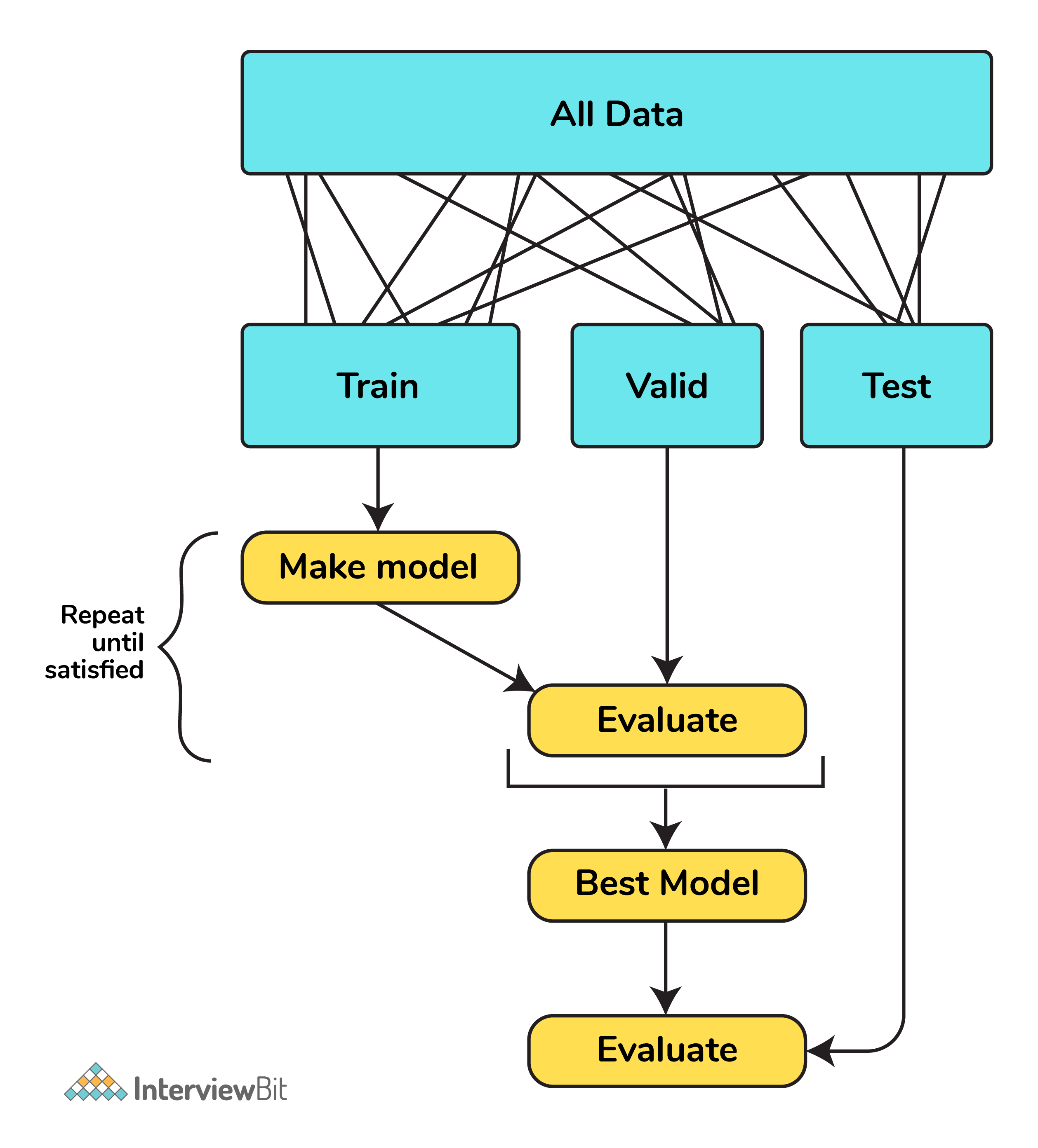
4. What is Cross-Validation?
Cross-validation is a method of splitting all your data into three parts: training, testing, and validation data. Data is split into k subsets, and the model has trained on k-1of those datasets.
The last subset is held for testing. This is done for each of the subsets. This is k-fold cross-validation. Finally, the scores from all the k-folds are averaged to produce the final score.
5. What are Different Kernels in SVM?
There are six types of kernels in SVM:
- Linear kernel - used when data is linearly separable.
- Polynomial kernel - When you have discrete data that has no natural notion of smoothness.
- Radial basis kernel - Create a decision boundary able to do a much better job of separating two classes than the linear kernel.
- Sigmoid kernel - used as an activation function for neural networks.
 Learn via our Video Courses
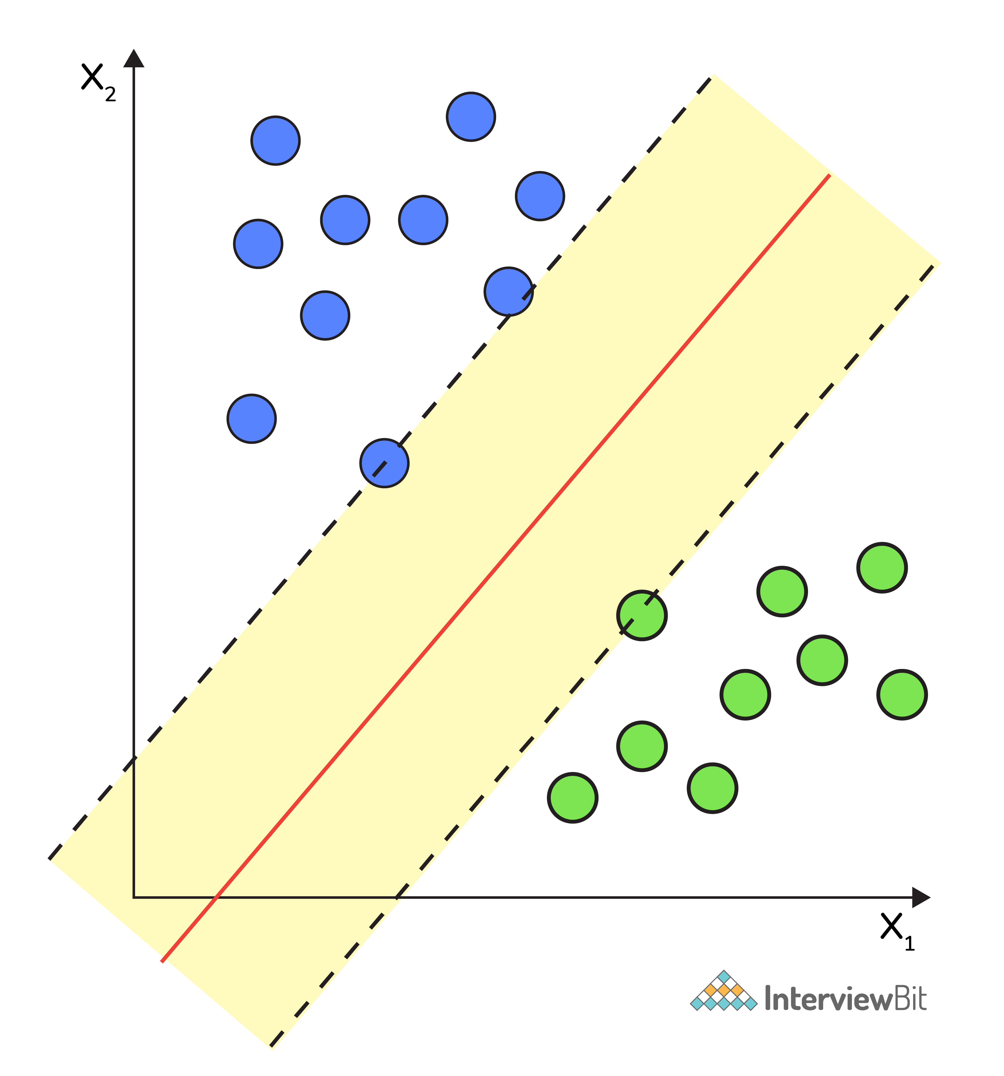
6. What are Support Vectors in SVM?
A Support Vector Machine (SVM) is an algorithm that tries to fit a line (or plane or hyperplane) between the different classes that maximizes the distance from the line to the points of the classes.
In this way, it tries to find a robust separation between the classes. The Support Vectors are the points of the edge of the dividing hyperplane as in the below figure.
7. What is PCA? When do you use it?
Principal component analysis (PCA) is most commonly used for dimension reduction.
In this case, PCA measures the variation in each variable (or column in the table). If there is little variation, it throws the variable out, as illustrated in the figure below:

Thus making the dataset easier to visualize. PCA is used in finance, neuroscience, and pharmacology.
It is very useful as a preprocessing step, especially when there are linear correlations between features.

 Real-Life Problems
 Detailed reports
8. What are Different Types of Machine Learning algorithms?
There are various types of machine learning algorithms. Here is the list of them in a broad category based on:
- Whether they are trained with human supervision (Supervised, unsupervised, reinforcement learning)
- The criteria in the below diagram are not exclusive, we can combine them any way we like.

9. What is Supervised Learning?
Supervised learning is a machine learning algorithm of inferring a function from labeled training data. The training data consists of a set of training examples.
Example: 01
Knowing the height and weight identifying the gender of the person. Below are the popular supervised learning algorithms.
- Support Vector Machines
- Regression
- Naive Bayes
- Decision Trees
- K-nearest Neighbour Algorithm and Neural Networks.
Example: 02
If you build a T-shirt classifier, the labels will be “this is an S, this is an M and this is L”, based on showing the classifier examples of S, M, and L.
10. What is Unsupervised Learning?
Unsupervised learning is also a type of machine learning algorithm used to find patterns on the set of data given. In this, we don’t have any dependent variable or label to predict. Unsupervised Learning Algorithms:
- Clustering,
- Anomaly Detection,
- Neural Networks and Latent Variable Models.
Example:
In the same example, a T-shirt clustering will categorize as “collar style and V neck style”, “crew neck style” and “sleeve types”.
11. What is ‘Naive’ in a Naive Bayes?
The Naive Bayes method is a supervised learning algorithm, it is naive since it makes assumptions by applying Bayes’ theorem that all attributes are independent of each other.
Bayes’ theorem states the following relationship, given class variable y and dependent vector x1 through xn:
P(yi | x1,..., xn) =P(yi)P(x1,..., xn | yi)(P(x1,..., xn)
Using the naive conditional independence assumption that each xiis independent: for all I this relationship is simplified to:
P(xi | yi, x1, ..., xi-1, xi+1, ...., xn) = P(xi | yi)
Since, P(x1,..., xn) is a constant given the input, we can use the following classification rule:
P(yi | x1, ..., xn) = P(y) ni=1P(xi | yi)P(x1,...,xn) and we can also use Maximum A Posteriori (MAP) estimation to estimate P(yi)and P(yi | xi) the former is then the relative frequency of class yin the training set.
P(yi | x1,..., xn) P(yi) ni=1P(xi | yi)
y = arg max P(yi)ni=1P(xi | yi)
The different naive Bayes classifiers mainly differ by the assumptions they make regarding the distribution of P(yi | xi): can be Bernoulli, binomial, Gaussian, and so on.
12. Explain SVM Algorithm in Detail
A Support Vector Machine (SVM) is a very powerful and versatile supervised machine learning model, capable of performing linear or non-linear classification, regression, and even outlier detection.
Suppose we have given some data points that each belong to one of two classes, and the goal is to separate two classes based on a set of examples.
In SVM, a data point is viewed as a p-dimensional vector (a list of p numbers), and we wanted to know whether we can separate such points with a (p-1)-dimensional hyperplane. This is called a linear classifier.
There are many hyperplanes that classify the data. To choose the best hyperplane that represents the largest separation or margin between the two classes.
If such a hyperplane exists, it is known as a maximum-margin hyperplane and the linear classifier it defines is known as a maximum margin classifier. The best hyperplane that divides the data in H3
We have data (x1, y1), ..., (xn, yn), and different features (xii, ..., xip), and yiis either 1 or -1.
The equation of the hyperplane H3 is the set of points satisfying:
w. x-b = 0
Where w is the normal vector of the hyperplane. The parameter b||w||determines the offset of the hyperplane from the original along the normal vector w
So for each i, either xiis in the hyperplane of 1 or -1. Basically, xisatisfies:
w . xi - b = 1 or w. xi - b = -1

Advanced Machine Learning Questions
1. What is F1 score? How would you use it?
Let’s have a look at this table before directly jumping into the F1 score.
| Prediction | Predicted Yes | Predicted No |
|---|---|---|
| Actual Yes | True Positive (TP) | False Negative (FN) |
| Actual No | False Positive (FP) | True Negative (TN) |
In binary classification we consider the F1 score to be a measure of the model’s accuracy. The F1 score is a weighted average of precision and recall scores.
F1 = 2TP/2TP + FP + FN
We see scores for F1 between 0 and 1, where 0 is the worst score and 1 is the best score.
The F1 score is typically used in information retrieval to see how well a model retrieves relevant results and our model is performing.
2. Define Precision and Recall?
Precision and recall are ways of monitoring the power of machine learning implementation. But they often used at the same time.
Precision answers the question, “Out of the items that the classifier predicted to be relevant, how many are truly relevant?”
Whereas, recall answers the question, “Out of all the items that are truly relevant, how many are found by the classifier?
In general, the meaning of precision is the fact of being exact and accurate. So the same will go in our machine learning model as well. If you have a set of items that your model needs to predict to be relevant. How many items are truly relevant?
The below figure shows the Venn diagram that precision and recall.
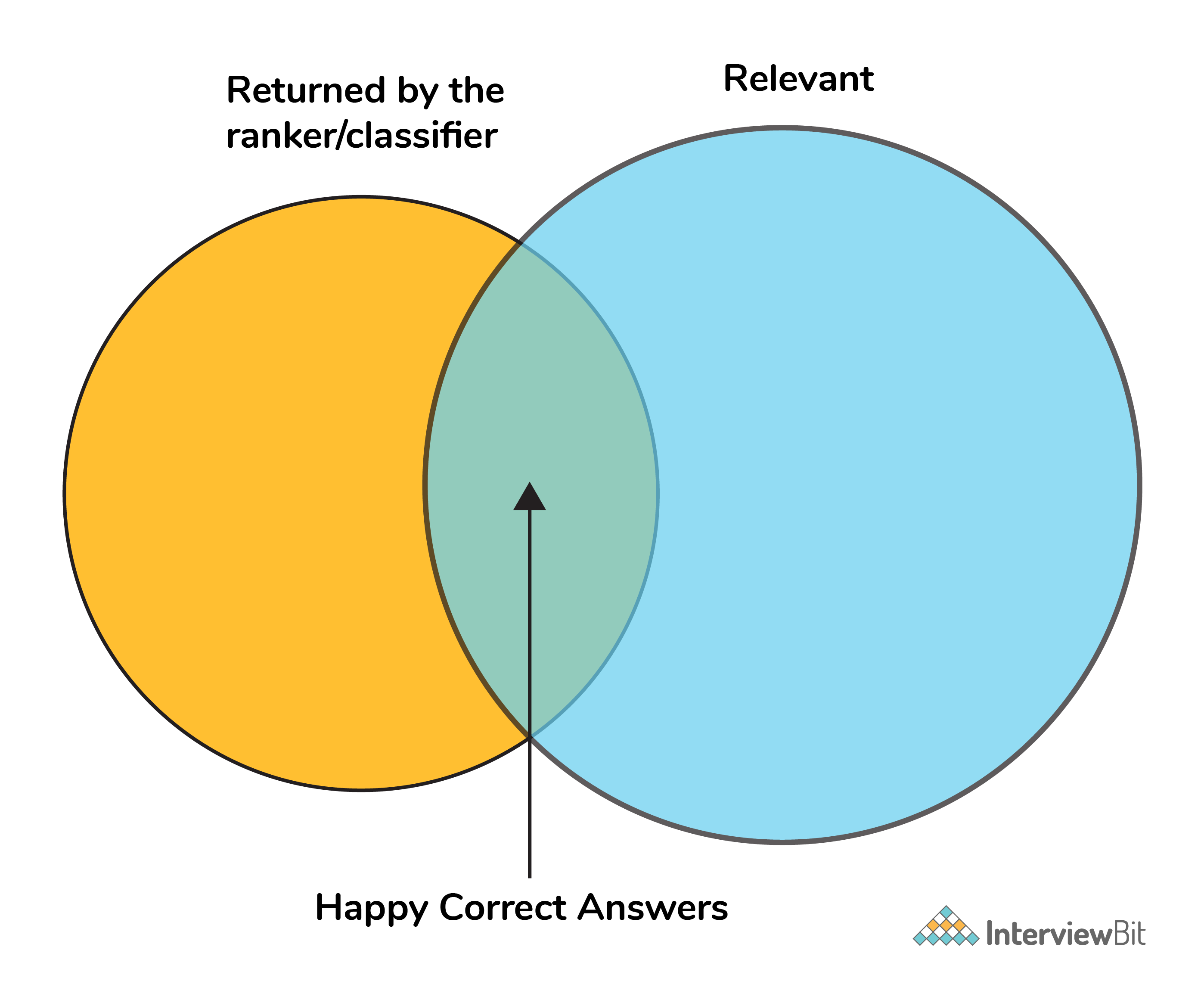
Mathematically, precision and recall can be defined as the following:
precision = # happy correct answers/# total items returned by ranker
recall = # happy correct answers/# total relevant answers
3. How to Tackle Overfitting and Underfitting?
Overfitting means the model fitted to training data too well, in this case, we need to resample the data and estimate the model accuracy using techniques like k-fold cross-validation.
Whereas for the Underfitting case we are not able to understand or capture the patterns from the data, in this case, we need to change the algorithms, or we need to feed more data points to the model.
4. What is a Neural Network?
It is a simplified model of the human brain. Much like the brain, it has neurons that activate when encountering something similar.
The different neurons are connected via connections that help information flow from one neuron to another.
5. What are Loss Function and Cost Functions? Explain the key Difference Between them?
When calculating loss we consider only a single data point, then we use the term loss function.
Whereas, when calculating the sum of error for multiple data then we use the cost function. There is no major difference.
In other words, the loss function is to capture the difference between the actual and predicted values for a single record whereas cost functions aggregate the difference for the entire training dataset.
The Most commonly used loss functions are Mean-squared error and Hinge loss.
Mean-Squared Error(MSE): In simple words, we can say how our model predicted values against the actual values.
Hinge loss: It is used to train the machine learning classifier, which is
L(y) = max(0,1- yy)
Where y = -1 or 1 indicating two classes and y represents the output form of the classifier. The most common cost function represents the total cost as the sum of the fixed costs and the variable costs in the equation y = mx + b
6. What is Ensemble learning?
Ensemble learning is a method that combines multiple machine learning models to create more powerful models.
There are many reasons for a model to be different. Few reasons are:
- Different Population
- Different Hypothesis
- Different modeling techniques
When working with the model’s training and testing data, we will experience an error. This error might be bias, variance, and irreducible error.
Now the model should always have a balance between bias and variance, which we call a bias-variance trade-off.
This ensemble learning is a way to perform this trade-off.
There are many ensemble techniques available but when aggregating multiple models there are two general methods:
- Bagging, a native method: take the training set and generate new training sets off of it.
- Boosting, a more elegant method: similar to bagging, boosting is used to optimize the best weighting scheme for a training set.
7. How do you make sure which Machine Learning Algorithm to use?
It completely depends on the dataset we have. If the data is discrete we use SVM. If the dataset is continuous we use linear regression.
So there is no specific way that lets us know which ML algorithm to use, it all depends on the exploratory data analysis (EDA).
EDA is like “interviewing” the dataset; As part of our interview we do the following:
- Classify our variables as continuous, categorical, and so forth.
- Summarize our variables using descriptive statistics.
- Visualize our variables using charts.
Based on the above observations select one best-fit algorithm for a particular dataset.
8. How to Handle Outlier Values?
An Outlier is an observation in the dataset that is far away from other observations in the dataset. Tools used to discover outliers are
- Box plot
- Z-score
- Scatter plot, etc.
Typically, we need to follow three simple strategies to handle outliers:
- We can drop them.
- We can mark them as outliers and include them as a feature.
- Likewise, we can transform the feature to reduce the effect of the outlier.
9. What is a Random Forest? How does it work?
Random forest is a versatile machine learning method capable of performing both regression and classification tasks.
Like bagging and boosting, random forest works by combining a set of other tree models. Random forest builds a tree from a random sample of the columns in the test data.
Here’s are the steps how a random forest creates the trees:
- Take a sample size from the training data.
- Begin with a single node.
- Run the following algorithm, from the start node:
- If the number of observations is less than node size then stop.
- Select random variables.
- Find the variable that does the “best” job of splitting the observations.
- Split the observations into two nodes.
- Call step `a` on each of these nodes.
10. What is Collaborative Filtering? And Content-Based Filtering?
Collaborative filtering is a proven technique for personalized content recommendations. Collaborative filtering is a type of recommendation system that predicts new content by matching the interests of the individual user with the preferences of many users.
Content-based recommender systems are focused only on the preferences of the user. New recommendations are made to the user from similar content according to the user’s previous choices.

11. What is Clustering?
Clustering is the process of grouping a set of objects into a number of groups. Objects should be similar to one another within the same cluster and dissimilar to those in other clusters.
A few types of clustering are:
- Hierarchical clustering
- K means clustering
- Density-based clustering
- Fuzzy clustering, etc.
12. How can you select K for K-means Clustering?
There are two kinds of methods that include direct methods and statistical testing methods:
- Direct methods: It contains elbow and silhouette
- Statistical testing methods: It has gap statistics.
The silhouette is the most frequently used while determining the optimal value of k.
13. What are Recommender Systems?
A recommendation engine is a system used to predict users’ interests and recommend products that are quite likely interesting for them.
Data required for recommender systems stems from explicit user ratings after watching a film or listening to a song, from implicit search engine queries and purchase histories, or from other knowledge about the users/items themselves.
14. How do check the Normality of a dataset?
Visually, we can use plots. A few of the normality checks are as follows:
- Shapiro-Wilk Test
- Anderson-Darling Test
- Martinez-Iglewicz Test
- Kolmogorov-Smirnov Test
- D’Agostino Skewness Test
15. Can logistic regression use for more than 2 classes?
No, by default logistic regression is a binary classifier, so it cannot be applied to more than 2 classes. However, it can be extended for solving multi-class classification problems (multinomial logistic regression)
16. Explain Correlation and Covariance?
Correlation is used for measuring and also for estimating the quantitative relationship between two variables. Correlation measures how strongly two variables are related. Examples like, income and expenditure, demand and supply, etc.
Covariance is a simple way to measure the correlation between two variables. The problem with covariance is that they are hard to compare without normalization.
17. What is P-value?
P-values are used to make a decision about a hypothesis test. P-value is the minimum significant level at which you can reject the null hypothesis. The lower the p-value, the more likely you reject the null hypothesis.
18. What are Parametric and Non-Parametric Models?
Parametric models will have limited parameters and to predict new data, you only need to know the parameter of the model.
Non-Parametric models have no limits in taking a number of parameters, allowing for more flexibility and to predict new data. You need to know the state of the data and model parameters.
19. What is Reinforcement Learning?
Reinforcement learning is different from the other types of learning like supervised and unsupervised. In reinforcement learning, we are given neither data nor labels. Our learning is based on the rewards given to the agent by the environment.
20. Difference Between Sigmoid and Softmax functions?
The sigmoid function is used for binary classification. The probabilities sum needs to be 1. Whereas, Softmax function is used for multi-classification. The probabilities sum will be 1.
Conclusion
The above-listed questions are the basics of machine learning. Machine learning is advancing so fast hence new concepts will emerge. So to get up to date with that join communities, attend conferences, read research papers. By doing so you can crack any ML interview.
Additional Resources
- Practice Coding
- Best Machine Learning Courses
- Best Data Science Courses
- Free Deep Learning Course with Certification
- Python Interview Questions
- AI MCQs
- Machine Learning Engineer: Career Guide
- Deep Learning Interview
- Machine Learning Engineer Salary
- Machine Learning Vs Data Science
- Machine Learning Vs Deep Learning
- Difference Between Artificial Intelligence and Machine Learning
- Additional 100+ Machine Learning Interview Questions and Answers
Machine Learning Important Questions
1. What is feature engineering? What are the most important techniques?
Raw data is rarely in a shape that machine learning models can learn from effectively. Feature engineering is the process of transforming that raw data into inputs that actually carry signal, and in practice, it often has more impact on model performance than algorithm choice does.
The most important techniques are:
1. Handling missing values - dropping rows works only when missingness is rare. Otherwise, impute using mean or median for numerical features and mode for categoricals. For more complex patterns, KNN imputation or iterative imputers like MICE give better results.
2. Encoding categoricals - one-hot encoding works well for low-cardinality features. Label encoding suits ordinal data. Target encoding replaces categories with the mean target value and is particularly effective for high-cardinality features like city or product ID.
3. Feature scaling - StandardScaler normalizes to zero mean and unit variance. MinMaxScaler compresses values to a fixed range. Distance-based models like KNN and SVMs are sensitive to scale; tree-based models are not.
4. Log and power transforms - skewed distributions hurt linear models. Applying a log transform to features like income or page views brings them closer to normal and stabilizes variance.
5. Date and time decomposition - extracting hour, day of week, month, or is_weekend from a timestamp often reveals patterns that the raw timestamp alone cannot.
6, Feature selection - correlation analysis removes redundant features, mutual information captures non-linear relationships, and SHAP values identify which features actually drive model predictions.
2. What are ensemble methods? Compare bagging (Random Forest) vs boosting (XGBoost).
Ensemble methods combine multiple models to produce a result that is more accurate and robust than any single model could achieve alone. The core idea is that individual models each make different mistakes, and combining them carefully averages those mistakes out.
Bagging, short for bootstrap aggregating, trains multiple models in parallel, each on a different random sample of the training data drawn with replacement. Because each model sees a slightly different dataset, they develop different biases, and averaging their predictions reduces overall variance. Random Forest is the most widely used bagging algorithm - it builds hundreds of decision trees, each trained on a bootstrap sample and a random subset of features, then aggregates their outputs. This randomness is deliberate; it prevents the trees from being too correlated with each other, which would defeat the purpose of combining them.
Boosting takes a different approach. Models are trained sequentially, where each new model focuses specifically on the examples the previous one got wrong. This process reduces bias rather than variance; the ensemble gradually corrects its own mistakes. AdaBoost was one of the first boosting algorithms, adjusting sample weights after each round. Gradient Boosting improved on this by framing the process as gradient descent in function space. XGBoost and LightGBM are optimized implementations of gradient boosting that add regularization, handle missing values natively, and are engineered for speed, which is why they dominate tabular data competitions on Kaggle and are a go-to in industry for structured data problems.
Beyond bagging and boosting, stacking trains a meta-learner on top of several base models, learning how to best combine their predictions. Voting classifiers take a simpler route, aggregating predictions by majority vote or averaging probabilities across models.
3. Explain the confusion matrix. What are precision, recall, F1-score, and AUC-ROC?
A confusion matrix breaks down a classifier's predictions into four outcomes: true positives, true negatives, false positives, and false negatives. Accuracy alone doesn't tell you much about imbalanced datasets, which is why these four cells matter.
Precision is TP/(TP+FP) - of everything the model predicted as positive, how many actually were? It matters when false positives are costly. A spam filter wrongly blocking legitimate emails is a real problem.
Recall is TP/(TP+FN) - of all actual positives, how many did the model catch? This is the priority when missing a positive is dangerous. A cancer screening model that misses cases is far more harmful than one that over-flags.
F1-score is the harmonic mean of precision and recall, useful when you need a single number that balances both, and the class distribution is uneven.
AUC-ROC plots the true positive rate against the false positive rate across all possible decision thresholds, not just the default 0.5. The area under that curve tells you how well the model separates classes overall. An AUC of 1.0 means perfect separation; 0.5 means the model is essentially guessing.
4. What is cross-validation? Why is k-fold preferred over a simple train/test split?
A single train/test split is unreliable; your evaluation score depends heavily on which data points ended up in the test set. K-fold removes that problem by rotating the test set across k different splits and averaging the results, so every data point gets tested exactly once.
Stratified k-fold goes a step further by preserving class distribution across folds, which is important for imbalanced datasets. For very small datasets, leave-one-out cross-validation uses a single sample as the test set each time, squeezing the most out of limited data.
One thing that breaks cross-validation is applying preprocessing to the full dataset before splitting. Information from the test fold leaks into training this way. Preprocessing must always happen inside each fold, which is why using a scikit-learn Pipeline is the right approach, not optional.
5. What is regularization? Compare L1 (Lasso) and L2 (Ridge) regularization.
When a model overfits, it is usually because it has assigned large weights to features that only matter in the training data. Regularization adds a penalty term to the loss function that discourages this, forcing the model to stay simpler and generalize better.
L1 regularization, or Lasso, penalizes the absolute value of weights and can push them all the way to zero, effectively removing features from the model. Geometrically, L1 creates a diamond-shaped constraint region in weight space. The sharp corners of that diamond sit on the axes, which means the optimal solution frequently lands exactly on one, zeroing out some weights entirely. This makes Lasso the right choice when you want the model to perform feature selection automatically.
L2 regularization, or Ridge, penalizes the square of weights instead. Its constraint region is a smooth sphere, which distributes the penalty evenly across all weights rather than eliminating any. This makes Ridge better suited for datasets where many correlated features each carry some signal.
When neither works well alone, ElasticNet combines both penalties, inheriting sparsity from L1 and the stability on correlated features from L2. It is particularly useful on high-dimensional datasets where some features are irrelevant, but others are heavily correlated.
6. What is gradient descent? Explain batch, mini-batch, and stochastic variants.
Gradient descent is the optimization algorithm that most machine learning models rely on to learn. What you need to keep in mind is that the model starts with random parameters, measures how wrong its predictions are using a loss function, and then adjusts those parameters step by step in the direction that reduces that error. The size of each step is controlled by the learning rate. Set it too high, and the model overshoots the minimum and never converges. Set it too low and training takes forever, sometimes getting stuck before reaching a good solution.
The three variants differ in how much data they use to compute each update.
Batch gradient descent uses the entire training dataset to calculate the gradient before making a single update. The direction it moves is accurate and stable, but on a dataset with millions of rows, this becomes slow and memory-heavy. It is rarely used in practice for large-scale problems.
Stochastic gradient descent, or SGD, goes to the other extreme; it updates parameters after every single training example. This makes it fast and gives it the ability to escape shallow local minima because of the noise in each update. The downside is that this same noise makes convergence erratic, and the loss curve jumps around rather than declining smoothly.
Mini-batch gradient descent splits the difference. It computes gradients on small batches, typically between 32 and 256 samples, and is the default choice in almost every modern ML workflow. It is fast enough for large datasets, stable enough to converge reliably, and plays well with GPU hardware. If you want more such questions in this area, try out Top Deep Learning Interview Questions and Answers
On top of this, optimizers like Adam improve on basic gradient descent by adapting the learning rate for each parameter individually and incorporating momentum to accelerate through flat regions of the loss surface. Vanishing and exploding gradients, where gradients shrink or blow up during backpropagation in deep networks, are handled through gradient clipping, careful weight initialization, and learning rate scheduling.
7. Explain the bias-variance tradeoff. How do underfitting and overfitting relate to it?
When a machine learning model makes predictions, its total error comes from two sources, bias and variance. Understanding what each one means and how they fight each other is key to diagnosing why a model isn't performing well.
Bias is the error that comes from a model being too simple for the problem. Imagine trying to predict house prices in Bangalore using only the number of bedrooms, ignoring location, age of the property, and nearby infrastructure. The model will miss important patterns, not just on new data, but on the training data too. That is underfitting. Training error is high, test error is high, and adding more data rarely helps because the model itself is the bottleneck.
Variance is the error that comes from a model being too sensitive to the training data. A deep decision tree trained on a small dataset will learn every quirk and outlier in that data as if it were a real pattern. It scores well on training data but struggles the moment it sees anything new. That is overfitting, low training error, and high test error.
Plot total error against model complexity, and you get a U-shaped curve. Simple models sit on the left with high bias. Complex models sit on the right with high variance. The lowest point of that curve is where you want to be.
The best way to understand what works in practicality here is to use a learning curve. If training and validation errors are both high, the model needs more complexity. If validation error is pulling away from training error, pull back with regularization, pruning, or more data. K-fold cross-validation gives a more reliable read on generalization than a single train-test split, especially on smaller datasets.
8. What is the difference between supervised, unsupervised, and reinforcement learning?
The three paradigms of machine learning differ in one fundamental way, and that is the nature of the data the model learns from.
Supervised learning uses labeled data where every input comes paired with the correct output. The model learns to map one to the other, then uses that mapping to make predictions on new data. This covers two types of tasks. Classification predicts discrete labels, like whether a loan applicant is likely to default or whether a medical scan shows signs of disease. Regression predicts continuous values, like forecasting tomorrow's air quality index or estimating delivery time on a Swiggy order. Algorithms like logistic regression, SVMs, and gradient boosted trees are workhorses of this category, and most production ML systems you interact with daily, credit scoring, spam filters, and search ranking, are supervised learning problems at their core.
Unsupervised learning works without any labels. The model's job isn't to predict a specific output; it's to find structure in the data that isn't immediately visible. Clustering algorithms like K-Means and DBSCAN group similar data points together. You can also see that Flipkart uses this kind of approach to segment customers by purchasing behavior and tailor recommendations accordingly. Dimensionality reduction techniques like PCA compress high-dimensional data into fewer, more meaningful features, which helps with visualization and makes downstream models faster and more efficient.
Reinforcement learning operates differently from both. There is no fixed dataset; instead, an agent takes actions inside an environment and receives rewards or penalties depending on what happens. Over thousands of iterations, it learns a policy that maximizes cumulative reward. Algorithms like Q-learning and PPO drive applications like game-playing AIs, robotics, and increasingly, the fine-tuning of large language models through human feedback, a technique known as RLHF. Going through more data sicence interview questions can give you some clarity as well.
Python Machine Learning Interview Questions
1. How do you save and load a trained ML model in Python for production deployment?
Training a model is only half the work, getting it into production reliably requires saving it correctly and thinking about how it will be served.import joblib
joblib.dump(pipeline, 'model_pipeline.joblib')
pipeline = joblib.load('model_pipeline.joblib')
Always save the full Pipeline, not just the model. If you save only the classifier, you have to manually apply preprocessing at inference time, which is how inconsistencies between training and production creep in.
Pickle works for generic Python objects, but is slower with large arrays and carries the same version risk as joblib a model saved with scikit-learn 1.2 may not load correctly on 1.4. Pinning your library versions in a requirements.txt or conda environment file is not optional in production.
For cross-framework deployment, serving a PyTorch or TensorFlow model in an environment that does not have those libraries installed, ONNX exports models into a standardized format that can run anywhere.
For teams managing multiple model versions, MLflow provides a model registry that tracks experiments, versions, and metadata, and integrates with serving infrastructure. Models can be served via Flask or FastAPI for lightweight APIs, or deployed directly to AWS SageMaker or GCP AI Platform for scalable cloud inference.
Joblib is the standard choice for scikit-learn models. It handles large NumPy arrays more efficiently than vanilla pickle and is straightforward to use:
2. What is data leakage in ML? What are the most common ways it occurs in Python code?
Data leakage happens when information from outside the training set influences the model during training or evaluation. The result is a model that looks accurate on paper but underperforms the moment it hits real data because it was unknowingly trained on information it should never have seen.
The most common way it happens in Python is fitting a scaler or encoder on the full dataset before splitting:
scaler = StandardScaler()
X_scaled = scaler.fit_transform(X)
X_train, X_test, y_train, y_test = train_test_split(X_scaled, y)
The scaler computes mean and variance using the entire dataset, including the test set. The model has indirectly seen test data before evaluation.
The fix is to fit only on training data:
X_train, X_test, y_train, y_test = train_test_split(X, y)
scaler = StandardScaler()
X_train_scaled = scaler.fit_transform(X_train)
X_test_scaled = scaler.transform(X_test)
Other common sources of leakage:
Target encoding before splitting - if you replace a categorical feature with the mean target value computed on the full dataset, the model learns from test labels during training.
Future data in time series - using tomorrow's values to predict today's outcome is a frequent mistake when the dataset is not sorted chronologically before splitting.
Including the target in features - columns that are direct proxies of the target, like a transaction status column when predicting fraud, inflates accuracy trivially.
The most reliable way to prevent leakage entirely is a scikit-learn Pipeline. Because the Pipeline fits all transformers inside each cross-validation fold, there is no opportunity for test data to influence preprocessing; it is enforced by design rather than left to the developer to remember.
3. How would you train and evaluate a classification model using scikit-learn? Walk through the code.
The process follows a consistent structure regardless of the dataset or algorithm - load, split, build a pipeline, train, and evaluate on held-out data.
Start with splitting the data:
from sklearn.model_selection import train_test_split
X_train, X_test, y_train, y_test = train_test_split(X, y, test_size=0.2, stratify=y, random_state=42)
Using stratify=y ensures class distribution is preserved across both splits, which matters for imbalanced datasets.
Next, build a Pipeline with a ColumnTransformer to handle mixed feature types:
from sklearn.pipeline import Pipeline
from sklearn.compose import ColumnTransformer
from sklearn.preprocessing import StandardScaler, OneHotEncoder
from sklearn.ensemble import RandomForestClassifier

preprocessor = ColumnTransformer([
    ('num', StandardScaler(), numerical_cols),
    ('cat', OneHotEncoder(), categorical_cols)
])

pipeline = Pipeline([
    ('preprocessor', preprocessor),
    ('classifier', RandomForestClassifier())
])
Fit on training data only, then evaluate on the test set:
pipeline.fit(X_train, y_train)
y_pred = pipeline.predict(X_test)

from sklearn.metrics import classification_report, roc_auc_score

print(classification_report(y_test, y_pred))
print(roc_auc_score(y_test, pipeline.predict_proba(X_test)[:,1]))
Never evaluate on training data, it tells you nothing about real-world performance.
For more robust evaluation, use StratifiedKFold with cross_val_score instead of a single split. For hyperparameter tuning, GridSearchCV searches exhaustively while RandomizedSearchCV is faster on large parameter spaces, both work directly on the pipeline, tuning preprocessing and model parameters together.
4. What is the difference between StandardScaler and MinMaxScaler? When do you skip scaling?
Both scalers bring features onto a comparable scale, but they do it differently and suit different situations.
StandardScaler transforms each feature to have zero mean and unit variance, which is commonly called z-score normalization. It works well when the data is roughly normally distributed and is the right choice for algorithms like SVM, logistic regression, and PCA, which are sensitive to the magnitude of features but not to a fixed range.
MinMaxScaler compresses values into a fixed range, typically 0 to 1. This is preferred for neural networks and KNN, where bounded inputs either speed up convergence or directly affect distance calculations. If your data has hard boundaries that carry meaning, pixel values in an image, for instance, MinMaxScaler preserves that structure better than StandardScaler.
The one case where you skip scaling entirely is tree-based models. Random Forest, XGBoost, and LightGBM split features based on thresholds, not magnitudes. Multiplying every value in a column by a constant does not change where the best split is, so scaling has no effect on their predictions and adds unnecessary complexity to the pipeline.
5. How does a scikit-learn Pipeline work? Why should you always use one?
A scikit-learn Pipeline chains preprocessing steps and a final model into a single object that behaves like any other estimator, you call fit once and it handles everything in order. Without a Pipeline, preprocessing and modeling are separate steps that are easy to apply incorrectly, especially during cross-validation.
There are three strong reasons to always use one:
- Prevents data leakage. During cross-validation, the
Pipelineensures every transformer, scalers, imputers, encoders, is fit only on the training fold and applied to the validation fold. If you scale before splitting, the scaler has already seen the validation data, and your evaluation metrics are quietly optimistic. - Simplifies code. Instead of manually calling
fitandtransformat every step, a singlepipeline.fithandles the entire sequence. During inference,pipeline.predictruns every preprocessing step automatically, no risk of forgetting a transformation in production. - Enables end-to-end grid search.
GridSearchCVcan tune parameters across all steps simultaneously, including preprocessing choices like imputation strategy or number of PCA components, not just model parameters.
For datasets with mixed feature types, ColumnTransformer applies different preprocessing to numerical and categorical columns and feeds the combined output into the Pipeline. FunctionTransformer wraps any custom Python function into a step that fits cleanly into the Pipeline. make_pipeline is a shorthand that builds a Pipeline without naming each step manually.
6. How do you handle missing values in a dataset before training an ML model in Python?
The right strategy depends on how much data is missing and what type of feature it is.
If missingness is small under 5%, dropping those rows is usually acceptable. If an entire column is mostly missing, dropping it makes more sense than trying to impute it.
For numerical features, SimpleImputer handles mean or median imputation. Median is generally safer when the feature is skewed, since mean gets pulled by outliers. For categorical features, mode imputation is the standard approach.
When missing values follow complex patterns, where missingness in one feature correlates with values in another, KNNImputer or IterativeImputer, which implements MICE, give better results than simple statistics. For time series data, forward-fill or backward-fill preserves temporal order rather than replacing values with a global statistic.
The most important rule, and a common interview trap, is that the imputer must be fit only on training data. Consider a dataset where you impute age using the mean calculated across the full dataset, that mean already includes information from your test set. When the model is evaluated, it has indirectly seen test data, which inflates your metrics. The clean way to prevent this is a scikit-learn Pipeline, which ensures every preprocessing step is fit inside each cross-validation fold automatically, with no leakage possible.
7. What are the most important Python libraries for machine learning? What does each do?
Python's ML stack doesn’t consist of just one thing. It's several libraries working together, each handling a different part of the pipeline.
NumPy is the base layer. Arrays, matrix operations, reshaping. You won't always write it directly but it's running underneath almost everything else.
Pandas is where most of the actual work happens before modeling. Messy columns, wrong data types, missing values, tables that need joining. Real data is rarely clean and this is where you sort that out. Honestly underestimated how much time this takes until you're actually in a project.
Scikit-learn for modeling. Same fit/predict structure regardless of the algorithm, which makes switching fast. Pipelines, cross-validation, grid search all built in. Most projects that don't need deep learning never leave this library.
Matplotlib when you need control over your plots. Seaborn when you just need a heatmap or distribution chart quickly during exploration without writing much.
PyTorch has become the default for deep learning, most new projects go straight to it. TensorFlow still around in older production systems mostly.
Order of operations is almost always the same. Pandas to get the data into shape, scikit-learn to model it, deep learning framework only when the problem genuinely needs one.