A probability distribution is a statistical function that describes all the possible values and likelihoods that a random variable can take within a given range. This range will be bounded between the minimum and maximum possible values, but precisely where the possible value is likely to be plotted on the probability distribution depends on several factors such as mean, median, variance, skewness, kurtosis, etc.

Types of Probability Distributions:

• Normal Distribution or Gaussian distribution

Normal distribution or Gaussian distribution is also known as the bell-shaped curve and is the most important and commonly used probability distribution in statistics. Though shapes and shifts vary as per the mean and variance of a distribution, normal distributions generally look like the following:

The probability density function of a normal distribution is given by:

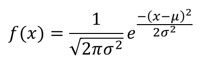
     Where: 

             𝝻 = mean of the distribution

             𝞂 = standard deviation of the distribution

Few observations to note about normal distribution:

(i) PDF of the distribution is symmetric around the mean.

(ii) The area under the bell curve is 1.

(iii) The mean, median, and mode of a normal distribution are equal.

(iv) 68% of the data points fall within one standard deviation from the mean, and 95% of the data points fall within two standard deviations from the mean. Refer to the diagram mentioned above.

• Bernoulli’s distribution

Distribution of a random variable that can have only two possible outcomes, usually 0 and 1. Probably the simplest of all, isn’t it? Then how can we interpret that? Let’s say there’s an event named A. The possible outcomes in a low level can be: either the event occurs or not. In real life, say a toss before any match. A team can either win or lose the toss. The failure can be denoted as 0 and 1 otherwise. Similarly, say you and I chose to team up against Thanos. In no parallel universe, I see a draw or negotiation. We will lose unless we make an infinity gauntlet. 

Now diving into more mathematics, Bernoulli’s distribution is a discrete probability distribution as its possible outcomes convey. So what we have here is a probability mass function instead of a probability density function. The PMF is given as:

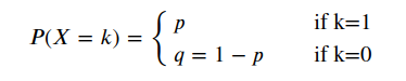
Where 0 < p < 1.

The mean of the probability distribution is p and the variance is p(1-p).

• Binomial Distribution

Distribution of random variable that represents the success in n trials with a probability of success p. Sounds confusing? Well, think of it as a combination of n Bernoulli distributions, each having a probability of success p, and independent of each other. In other words, Bernoulli’s distribution is nothing but a binomial distribution with a total number of trials as 1. Speaking of, Binomial Distribution is also discrete probability distribution, hence we’ll discuss the PMF. Before that, we must keep in mind that, in order for a random variable to follow a binomial distribution, it must adhere to certain rules or criteria as follows:

• Each trial must be independent of the other.
• The probability of success must be the same for every trial. 
• And there must be only two possible outcomes for each trial.

Now, coming to the PMF:

Where: X is the random variable, p is the probability of success in every trial, and q is the probability of failure i.e. q = 1 - p.  

The mean and variance of the distribution is np and np(1-p) respectively.

• Exponential Distribution

Time for a continuous distribution. Exponential distributions basically model the time elapsed between successive steps or events. Its parameter represents the speed of the process, the larger the faster the steeper. The real-world examples can be: time elapsed between the number of calls in a call center, the longevity of a car battery, even the changes you carry in your pocket approximately follows an exponential distribution (think about that).

Moving to the Probability density function as it is a continuous distribution:

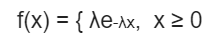
Where: λ is the distribution parameter. 

The mean and variance of the distribution are 1/λ and (1/λ)^2 respectively.

• Poisson Distribution

We discussed the time elapsed between events. Now think of counting the occurrences of events in an interval. Poisson Distribution kicks off an entrance here. It has certain assumptions such as:

• Any successful event should not influence the outcome of another successful event.
• The probability of success over a short interval must equal the probability of success over a longer interval.
• The probability of success in an interval approaches zero as the interval becomes smaller.

As it is a discrete distribution, it should have a PMF which can be formed as:

The mean and variance of the distribution are λ.

• Uniform Distribution

As the name suggests, every possible outcome is just equally likely. Say, for example, the outcome of a dice-roll. Each number from 1 to 6 is equally likely to appear. Now, moving to the density function:

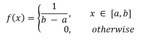
The mean and variance of the distribution would be (a+b)/2, and (b-a)^2/12 respectively.